Estimation of the reproduction number

written by Oswaldo Gressani

Introduction

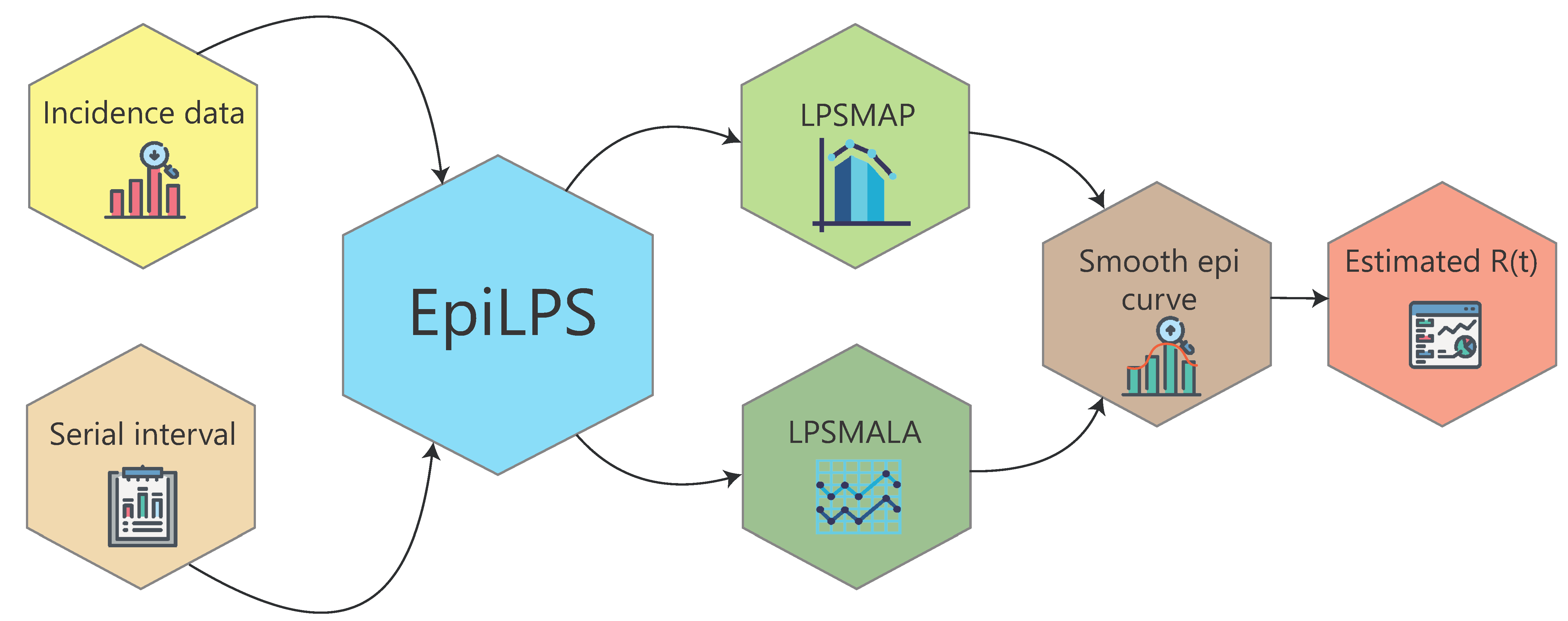
EpiLPS (Gressani et al. 2022) is the acronym for Epidemiological modeling (tool) with Laplacian-P-Splines. It proposes a new Bayesian methodology for estimating key epidemiological parameters. This documentation focuses on the estimation of the time-varying reproduction number \(\mathcal{R}_t\), i.e. the average number of secondary cases generated by an infectious agent at time \(t\); a key metric for assessing the transmission dynamics of an infectious disease and a useful reference for guiding interventions of governmental institutions in a public health crisis. The EpiLPS project builds upon two strong pillars in the statistical literature, namely Bayesian P-splines and Laplace approximations, to deliver a fast and flexible methodology for inference on \(\mathcal{R}_t\). EpiLPS requires two (external) inputs: (1) a time series of incidence counts and (2) a (discrete) serial interval distribution.

The underlying model for smoothing incidence counts is based on the negative binomial distribution to account for possible overdispersion in the data. EpiLPS has a two-phase engine for estimating \(\mathcal{R}_t\). First, Bayesian P-splines are used to smooth the epidemic curve and to compute estimates of the mean incidence count of the susceptible population at each day of the outbreak. Second, in the philosophy of Fraser (2007), the renewal equation is used as a bridge to link the estimated mean incidence and the reproduction number. As such, the second phase delivers a closed-form expression of \(\mathcal{R}_t\) as a function of the B-spline coefficients and the serial interval distribution.

Another key strength of EpiLPS is that two different strategies can be used to estimate \(\mathcal{R}_t\). The first approach called LPSMAP is completely sampling-free and fully relies on Laplace approximations and maximum a posteriori (MAP) computation of model hyperparameters for estimation. Routines for Laplace approximations and B-splines evaluations are typically the ones that are computationally most intensive and are therefore coded in C++ and integrated in R via the Rcpp package, making them time irrelevant. The second approach is called LPSMALA (Laplacian-P-splines with a Metropolis-adjusted Langevin algorithm) and is fully stochastic. It samples the posterior of the model by using Langevin diffusions in a Metropolis-within-Gibbs framework. Of course, LPSMAP has a computational advantage over LPSMALA. Thanks to the lightning fast implementation of Laplace approximations, LPSMAP typically delivers estimates of \(\mathcal{R}_t\) in a fraction of a second.

Fig 1. Idea behind EpiLPS.

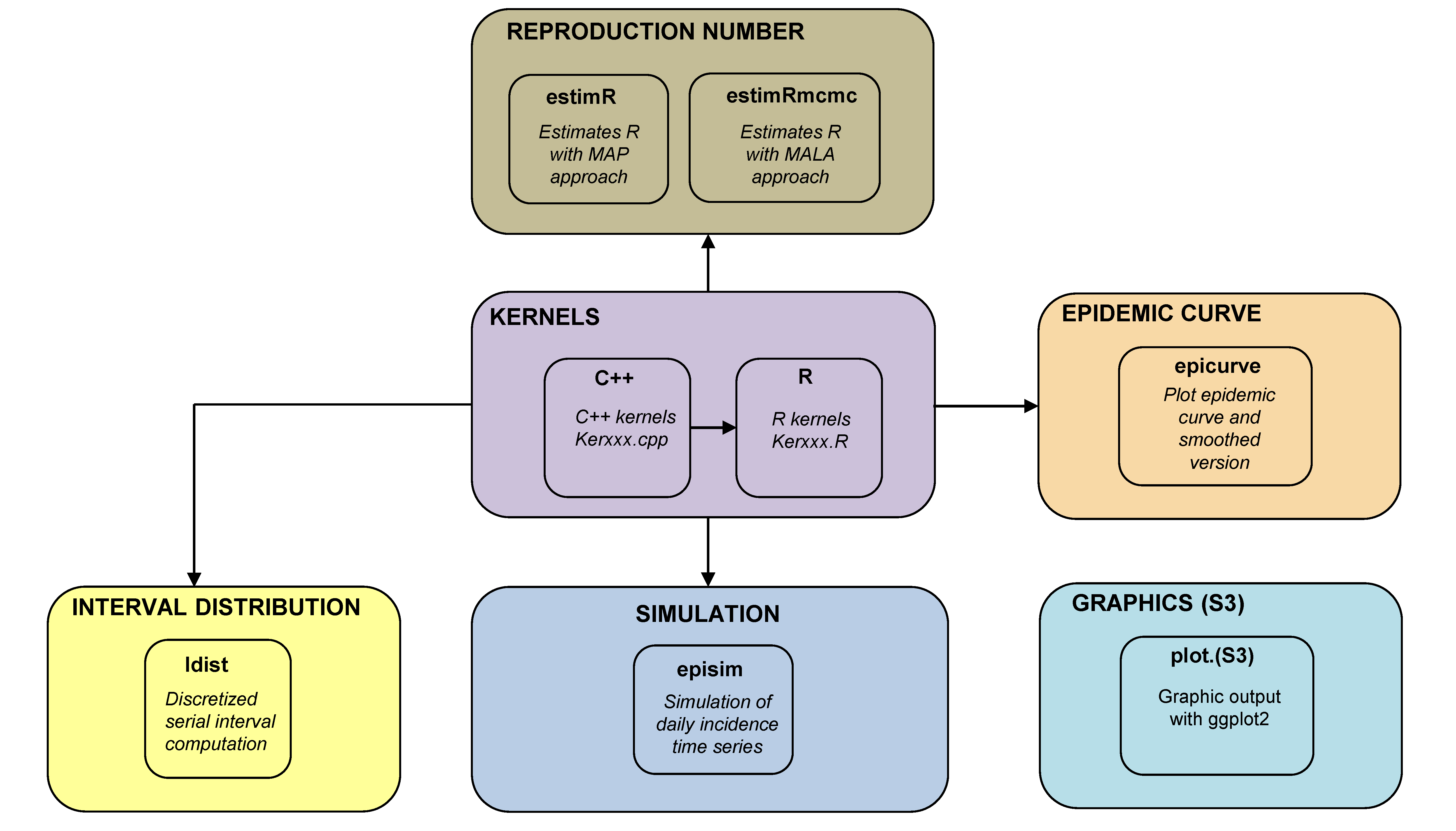
EpiLPS package architecture

The package has a modular architecture with simple routines aiming at an intuitive command input for users. Kernel routines (the machinery responsible for the hard computational work behind EpiLPS) are not directly surfaced to the user, i.e. they are not directly available in the package documentation but can be accessed by typing ls(getNamespace("EpiLPS"), all.names = TRUE) in the R console. All the routines starting with “Ker” are Kernel routines. These routines include (among others) likelihood evaluations, gradient and Hessian evaluations and posterior distribution evaluations.

The estimR() and estimRmcmc() routines can be used to estimate the time-varying reproduction number using Laplacian-P-splines with the MAP approach and MALA approach, respectively. The epicurve() function can be used to obtain a graphical representation of the epidemic curve (and its smoothed version), while the Idist() routine is meant to compute the (discrete) distribution of a disease interval, for instance the serial interval distribution to be used as an input in estimR(). Finally, there are some S3 methods available to summarize estimation results and an episim() routine to simulate time series of incidence data based on different functional patterns of the reproduction number over time.

Fig 2. High-level overview of the EpiLPS package.

EpiLPS GitHub repository

The associated GitHub repository https://github.com/oswaldogressani/EpiLPS hosts the in-development version before the associated stable version is released on CRAN https://cran.r-project.org/package=EpiLPS. To install the GitHub version of EpiLPS (with devtools) type the following lines in the R console:

install.packages("devtools")
devtools::install_github("oswaldogressani/EpiLPS")

Specification of a serial interval and data generation

To estimate \(\mathcal{R}_t\), EpiLPS requires a (discrete) serial interval distribution, i.e. a discrete probability distribution and a time series of incidence data. The Idist() function computes the probability density function and probability mass function for a disease interval based on the mean and standard deviation of the disease interval (expressed in days). The code below is used to obtain a (discrete) serial interval si for a given mean and standard deviation. By default these values are obtained by assuming a Gamma distribution for the disease interval, but the Weibull or LogNormal distributions can also be specified in the dist= option.

si_spec <- Idist(mean = 2.7, sd = 1.3, dist = "gamma")
si <- si_spec$pvec
si

##  [1] 0.1683155677 0.3309269357 0.2641722153 0.1416603809 0.0609478350
##  [6] 0.0228109990 0.0077559604 0.0024585172 0.0007387518 0.0002128371

plot(si_spec)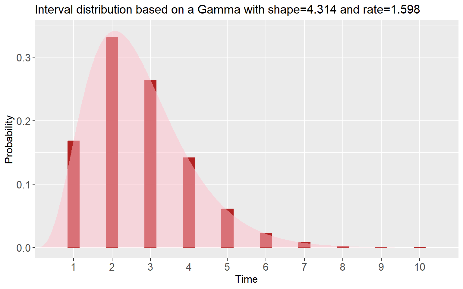

By calling plot() on the si_spec object, a plot of the serial interval is created with the discrete and continuous distribution. On top of that, the si_spec object also returns the (fitted) parameters for the chosen distribution of the disease interval that is also reflected in the plot title. Now, using the above serial interval, we can call the episim() routine to generate a time series of incidence data (say for an epidemic lasting 40 days). The data generating process (DGP) requires the specification of a functional form for the reproduction number (here we choose Rpattern = 5 among the six available patterns). A renewal equation model is used to generate the case incidence data based on a Poisson or negative binomial process (to be chosen by the user). Full details on the DGP can be found here https://doi.org/10.1371/journal.pcbi.1010618.s002.

set.seed(123)
datasim <- episim(si = si, Rpattern = 5, endepi = 40, dist = "negbin", overdisp = 15, plotsim = TRUE)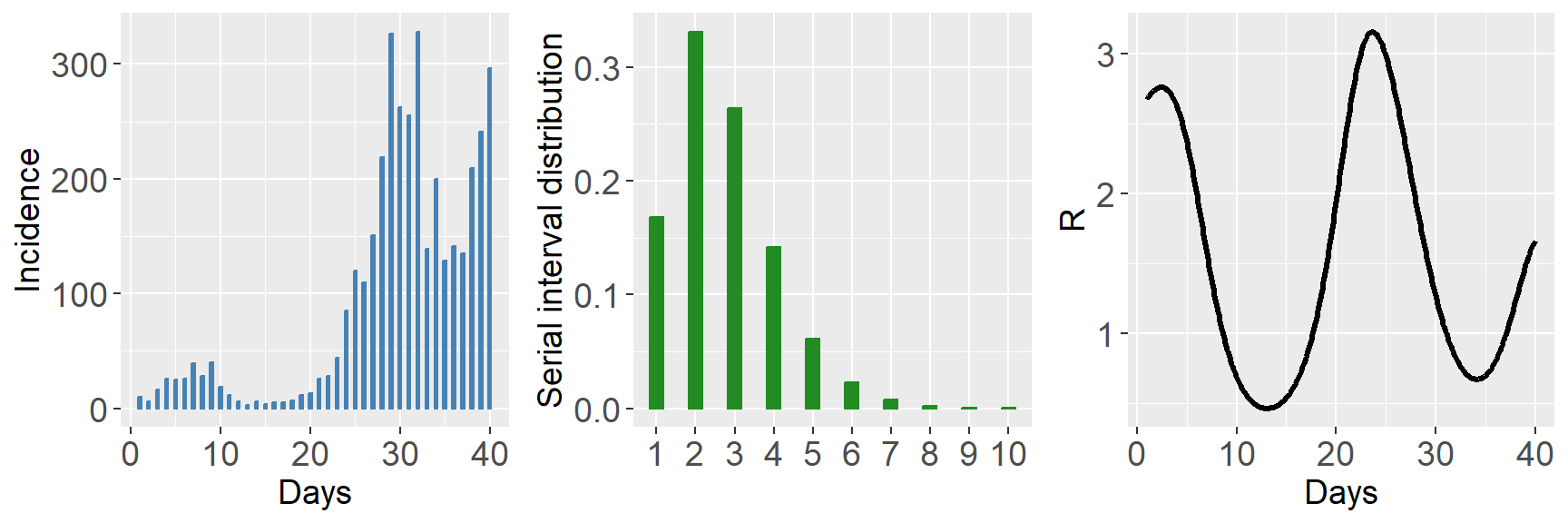

incidence <- datasim$y
incidence

##  [1]  10   6  16  26  25  26  39  28  40  19  12   6   3   6   4   5   5   7  12
## [20]  13  26  28  44  85 120 110 151 219 326 262 255 328 139 200 129 141 135 209
## [39] 241 296

By default, the number of cases at time \(t=1\) is fixed at 10. Specifying option plotsim = TRUE gives a summary plot of the generated data and the right panel gives the true underlying functional form of the reproduction number over the 40 days (as specified by Rpattern = 5). We now have a serial interval distribution and a time series of incidence data that can be used as inputs in the estimR() and estimRmcmcm() routines.

Estimation of the reproduction number

The estimR() and estimRmcmcm() are relatively simple to use with only a few inputs and intuitive outputs. Basically, both routines require a vector containing the incidence time series, a discrete serial interval distribution, a number of B-splines to be used in the basis (default is 30) and a vector of dates (optional). Another added value of these routines is that they also allow to compute the \(\mathcal{R}_t\) estimates using the Cori et al. (2013) and Wallinga and Teunis (2004) method, respectively. The code below defines an object called LPSfit from the estimR() routine. Actually, the latter object is a list with many different components summarizing the results of the fit. Among this list, the RLPS component is of particular interest as it gives a summary of the estimated reproduction number (point estimates and selected quantiles).

LPSfit <- estimR(incidence = incidence, si = si)
class(LPSfit)

## [1] "Rt"

knitr::kable(tail(LPSfit$RLPS[,1:7]))

	Time	R	Rsd	Rq0.025	Rq0.05	Rq0.25	Rq0.50
35	35	0.6419727	0.0324669	0.5815008	0.5908240	0.6204838	0.6419727
36	36	0.7212346	0.0376810	0.6511724	0.6619592	0.6963118	0.7212346
37	37	0.9116863	0.0455660	0.8267645	0.8398637	0.8815202	0.9116863
38	38	1.2018582	0.0529034	1.1026540	1.1180325	1.1667500	1.2018582
39	39	1.4957960	0.0603576	1.3821874	1.3998527	1.4556826	1.4957960
40	40	1.6824906	0.0903072	1.5148264	1.5406092	1.6227950	1.6824906

The estimR() routine generates an object of class Rt and there are two S3 methods associated with an object of that class, namely a summary() method and a plot() method. The former gives:

summary(LPSfit)

## Estimation of the reproduction number with Laplacian-P-splines 
## -------------------------------------------------------------- 
## Total number of days:          40 
## Routine time (seconds):        0.15 
## Method:                        Maximum a posteriori (MAP) 
## Hyperparam. optim method:      Nelder-Mead 
## Hyperparam. optim convergence: TRUE 
## Mean reproduction number:      1.346 
## Min  reproduction number:      0.312 
## Max  reproduction number:      2.651 
## --------------------------------------------------------------

This table give basic summary statistics related to the LPS fit (note how fast the routine is). Calling the S3 plot method yields a plot of the estimated reproduction number and associated 95% credible interval.

plot(LPSfit)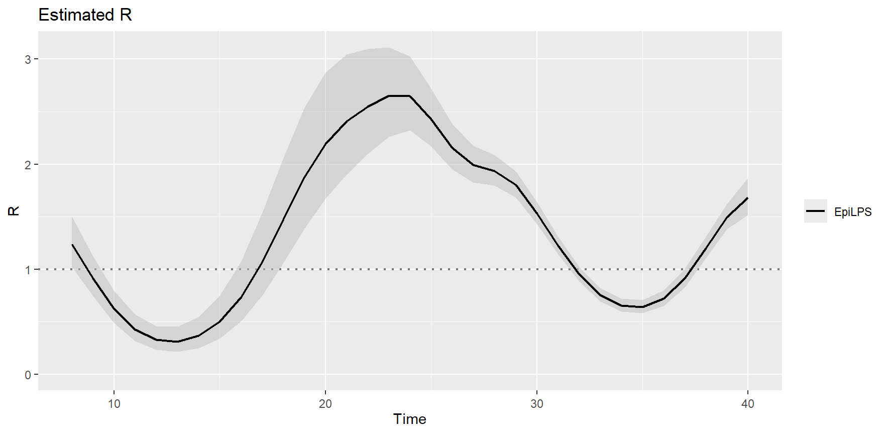

The estimRmcmcm() routine works similarly. By default it draws 5000 MCMC samples and uses a burn-in of size 2000. Being a fully stochastic approach, the latter routine is slower than estimR().

LPSfitmcmc <- estimRmcmc(incidence = incidence, si = si, niter = 5000, burnin = 2000)

summary(LPSfitmcmc)

## Estimation of the reproduction number with Laplacian-P-splines 
## -------------------------------------------------------------- 
## Total number of days:          40 
## Routine time (seconds):        1.8 
## Method:                        MCMC (with Langevin diffusion) 
## Hyperparam. optim method:      Nelder-Mead 
## Hyperparam. optim convergence: TRUE 
## Mean reproduction number:      1.359 
## Min  reproduction number:      0.314 
## Max  reproduction number:      2.715 
## --------------------------------------------------------------

The same exercise, but adding the Cori et al. (2013) EpiEstim fit. By specifying the addfit = "Cori" option in the S3 plot method, we can overlay both estimates.

LPSfit2 <- estimR(incidence = incidence, si = si, CoriR = TRUE)
knitr::kable(tail(LPSfit2$RCori[,1:7]))

	t_start	t_end	Mean(R)	Std(R)	Quantile.0.025(R)	Quantile.0.05(R)	Quantile.0.25(R)
28	29	35	1.0269038	0.0253576	0.9777996	0.9855533	1.0096885
29	30	36	0.8799678	0.0230693	0.8353282	0.8423690	0.8642998
30	31	37	0.8153488	0.0223740	0.7720809	0.7788991	0.8001483
31	32	38	0.8335788	0.0232811	0.7885677	0.7956581	0.8177601
32	33	39	0.8342298	0.0241325	0.7875957	0.7949362	0.8178283
33	34	40	1.0094248	0.0274527	0.9563291	0.9646975	0.9907751

plot(LPSfit2, addfit = "Cori")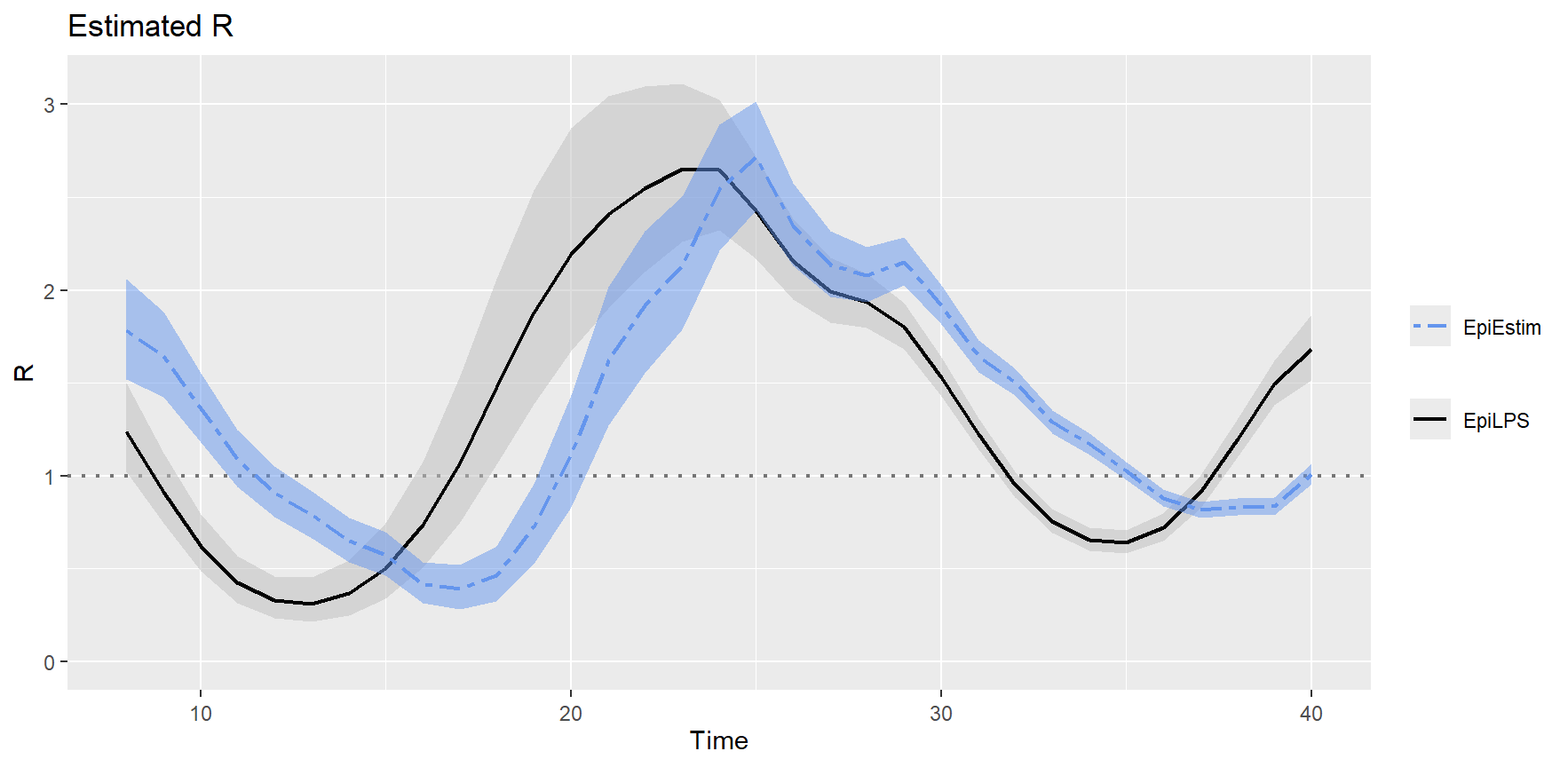

Of course, the estimated reproduction number can also be potted by extracting values from the LPSfit2 object in a traditional way as shown below. The interested reader can consult Gressani et al. (2022) for a detailed explanantion of the main differences between EpiEstim and EpiLPS.

tt <- seq(8, 40, by = 1)
Rtrue <- sapply(tt, datasim$Rtrue)
plot(tt, Rtrue, type = "l", xlab = "Time", ylab = "R", ylim = c(0,4),
     lwd = 2)
lines(tt, LPSfit2$RLPS$R[-(1:7)], col = "red", lwd = 2)
lines(tt, LPSfit2$RCori$`Mean(R)`, col = "blue", lwd = 2)
legend("topright", col = c("black","red","blue"), 
       c("True R","EpiLPS","EpiEstim"), bty = "n", lty = c(1,1,1))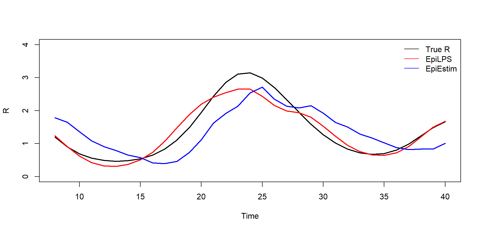

Customizing graphical output

EpiLPS uses ggplot2 to generate beautiful graphics and plots of the estimated reproduction number can be customized in various ways.

gridExtra::grid.arrange(
  plot(LPSfit, col = "firebrick", legendpos = "top", cicol = "orange"),
  plot(LPSfit, col = "forestgreen", legendpos = "none", cicol = "green",
       theme = "light", title = "Reproduction number"),
  plot(LPSfit, col = "darkblue", legendpos = "none", cicol = "orchid",
       theme = "classic"),
  plot(LPSfit, col = "white", legendpos = "none", cicol = "gray",
       theme = "dark"),
  nrow = 2, ncol = 2)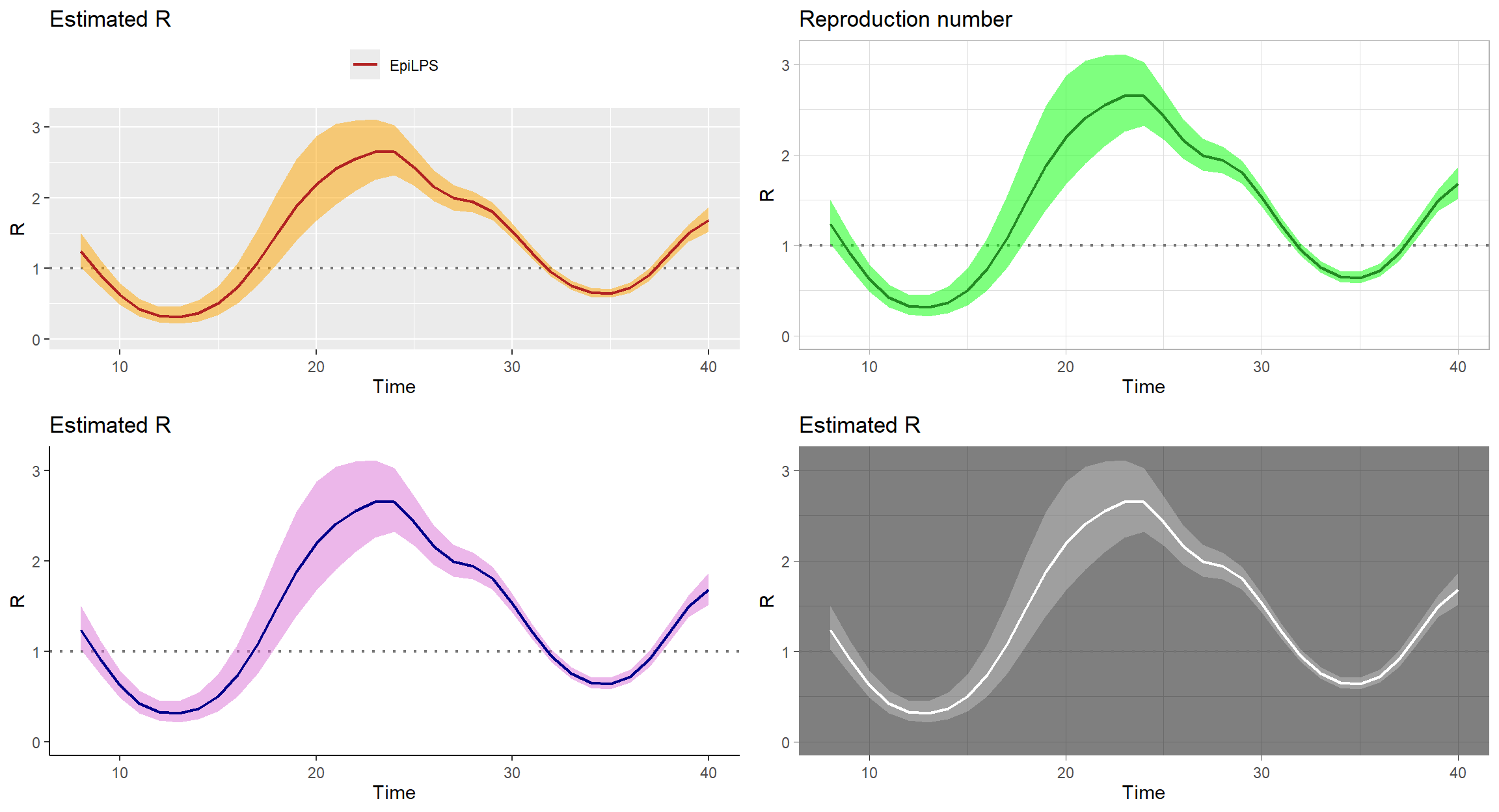

Illustration on the Zika virus in Girardot, Colombia (2015)

To illustrate EpiLPS on real data, we investigate the daily incidence of Zika virus disease in Girardot, Colombia from the outbreaks package. Incidence data is available from October 2015 to January 2016. First, the data is loaded and the epidemic curve is visualized with the epicurve() routine.

# Loading the data
zika <- zika_girardot_2015
plotIncidence <- epicurve(zika$cases, dates = zika$date, datelab = "14d", title = "Zika incidence")
plotIncidence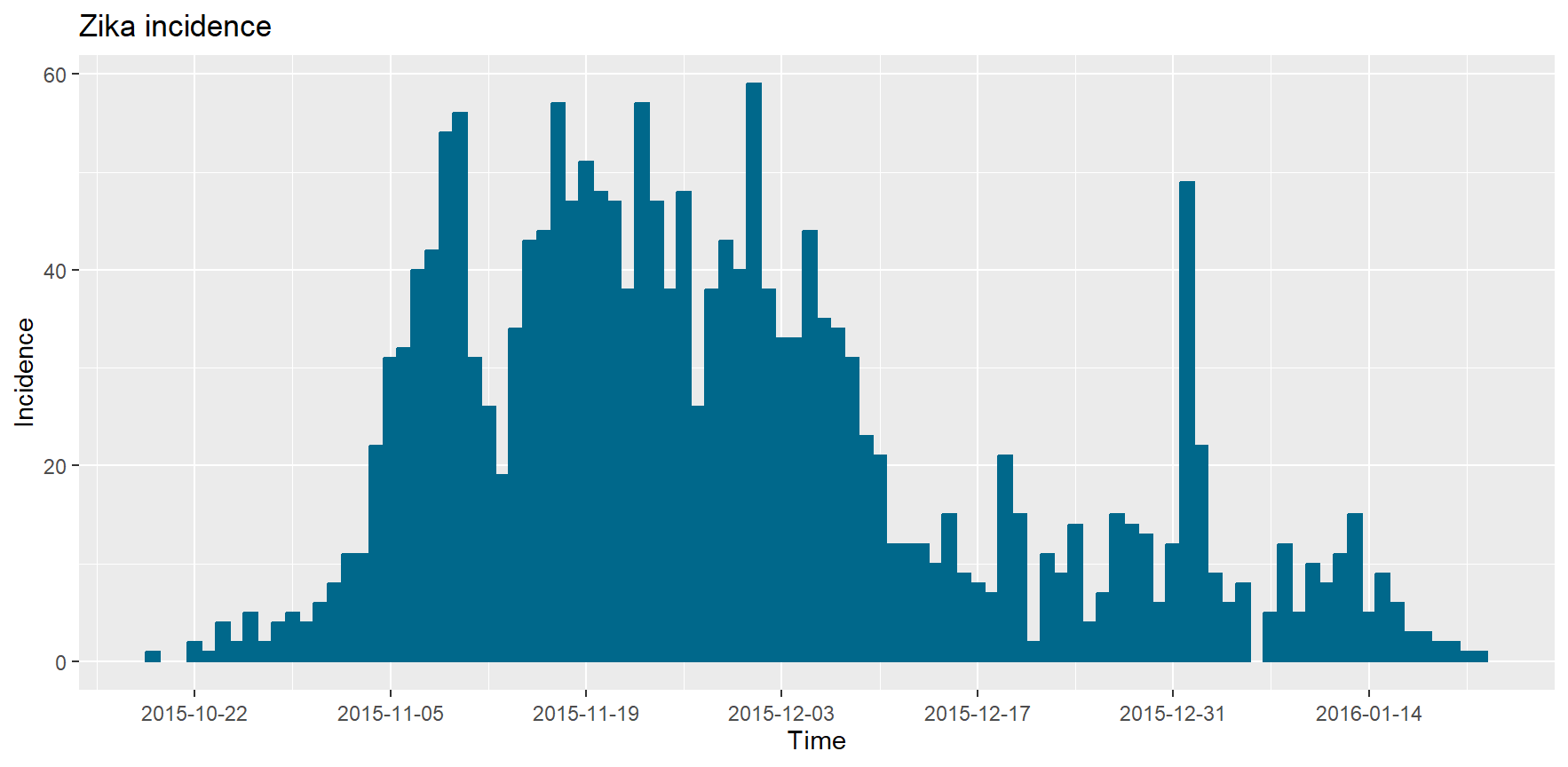

A serial interval distribution of mean 7 days (SD=1.5 days) is specified and the estimR() routine is used to estimate the reproduction number.

# Specification of the serial interval
si <- Idist(mean = 7, sd = 1.5)
siplot <- plot(si, titlesize = 11)
epifit <- estimR(zika$cases, dates = zika$date, si = si$pvec)
summary(epifit)

## Estimation of the reproduction number with Laplacian-P-splines 
## -------------------------------------------------------------- 
## Total number of days:          93 
## Routine time (seconds):        0.07 
## Method:                        Maximum a posteriori (MAP) 
## Hyperparam. optim method:      Nelder-Mead 
## Hyperparam. optim convergence: TRUE 
## Mean reproduction number:      1.355 
## Min  reproduction number:      0.177 
## Max  reproduction number:      5.047 
## --------------------------------------------------------------

Next, the estimation results are summarized into a single plot.

# Plot the smoothed epidemic curve
plotsmooth <- epicurve(zika$cases, dates = zika$date, datelab = "14d", smooth = epifit, smoothcol = "orange", title = "Zika incidence (smoothed)")

# Plot of the estimated reproduction number
Rplot <- plot(epifit, datelab = "7d", xtickangle = 70, legendpos = "none", col = "forestgreen")

# Show all plots together
gridExtra::grid.arrange(plotIncidence, plotsmooth, siplot, Rplot, nrow = 2, ncol = 2)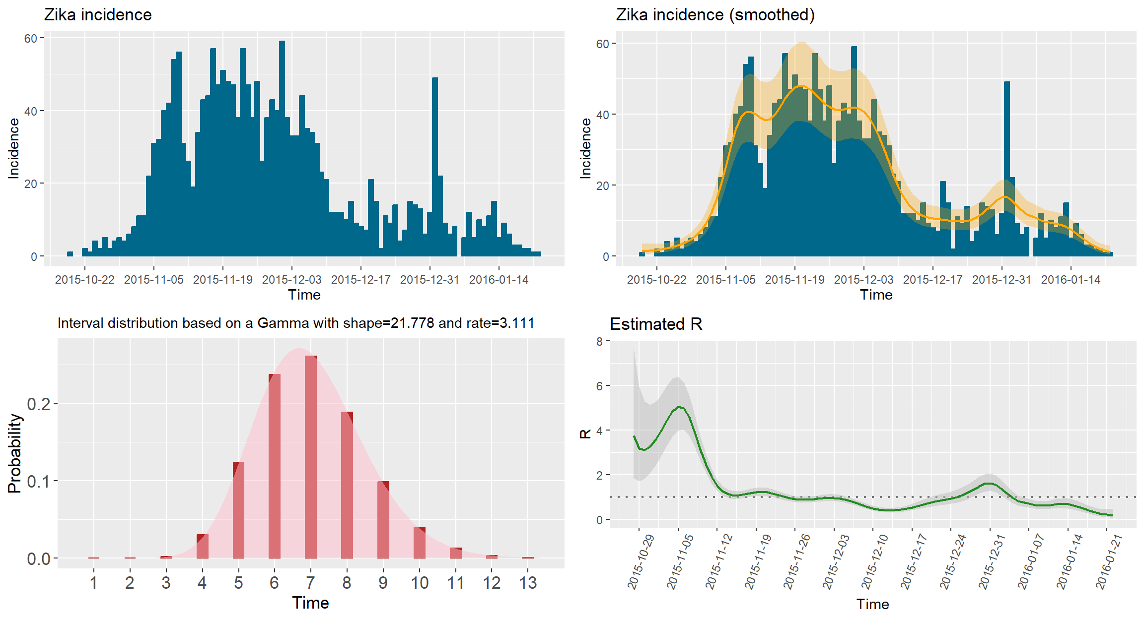

Illustration on outbreaks considered in Cori et al. (2013)

Data on the measles epidemic in Germany (1861)

data("Measles1861")
measlesDAT <- Measles1861
measles_incid <- measlesDAT$incidence
measles_si <- measlesDAT$si_distr
epifit_measles <- estimR(measles_incid, si = measles_si, CoriR = T)
epicurve_measles<- epicurve(measles_incid, datelab = "1d", title = "Measles, Hagelloch, Germany, 1861",
                            col = "lightblue3", smooth = epifit_measles, smoothcol = "dodgerblue4")
Rplot_measles <- plot(epifit_measles, timecut = 6, legendpos = "none")
Rplot_measles2 <- plot(epifit_measles, addfit = "Cori", timecut = 6, legendpos = "top")
siplot_measles <- plot(Idist(probs = measles_si), barcol = "dodgerblue", xtitlesize = 10)
gridExtra::grid.arrange(epicurve_measles, Rplot_measles, Rplot_measles2, 
                        siplot_measles, nrow = 2, ncol = 2)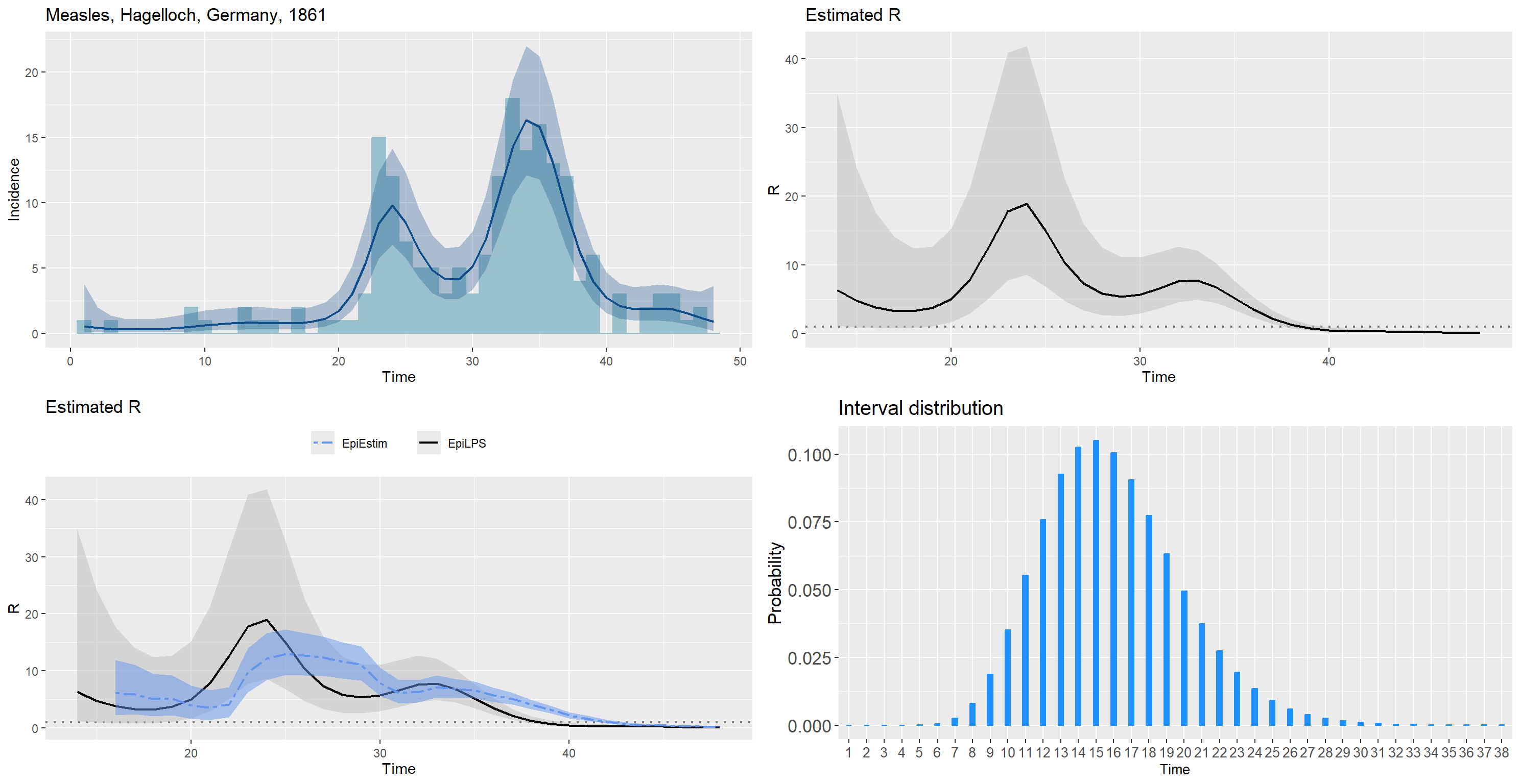

Influenza pandemic in Baltimore (1918)

data("Flu1918")
fluDAT <- Flu1918
flu_incid <- fluDAT$incidence
flu_si <- fluDAT$si_distr[-1]
epifit_flu <- estimR(flu_incid, si = flu_si, CoriR = T)
epicurve_flu <- epicurve(flu_incid, datelab = "7d", title = "Influenza, Baltimore, 1918",
                            col = "orange", smooth = epifit_flu, smoothcol = "firebrick")
Rplot_flu <- plot(epifit_flu, legendpos = "none")
Rplot_flu2 <- plot(epifit_flu, addfit = "Cori", legendpos = "top")
siplot_flu <- plot(Idist(probs = flu_si), barcol = "indianred1")
gridExtra::grid.arrange(epicurve_flu, Rplot_flu, Rplot_flu2, 
                        siplot_flu, nrow = 2, ncol = 2)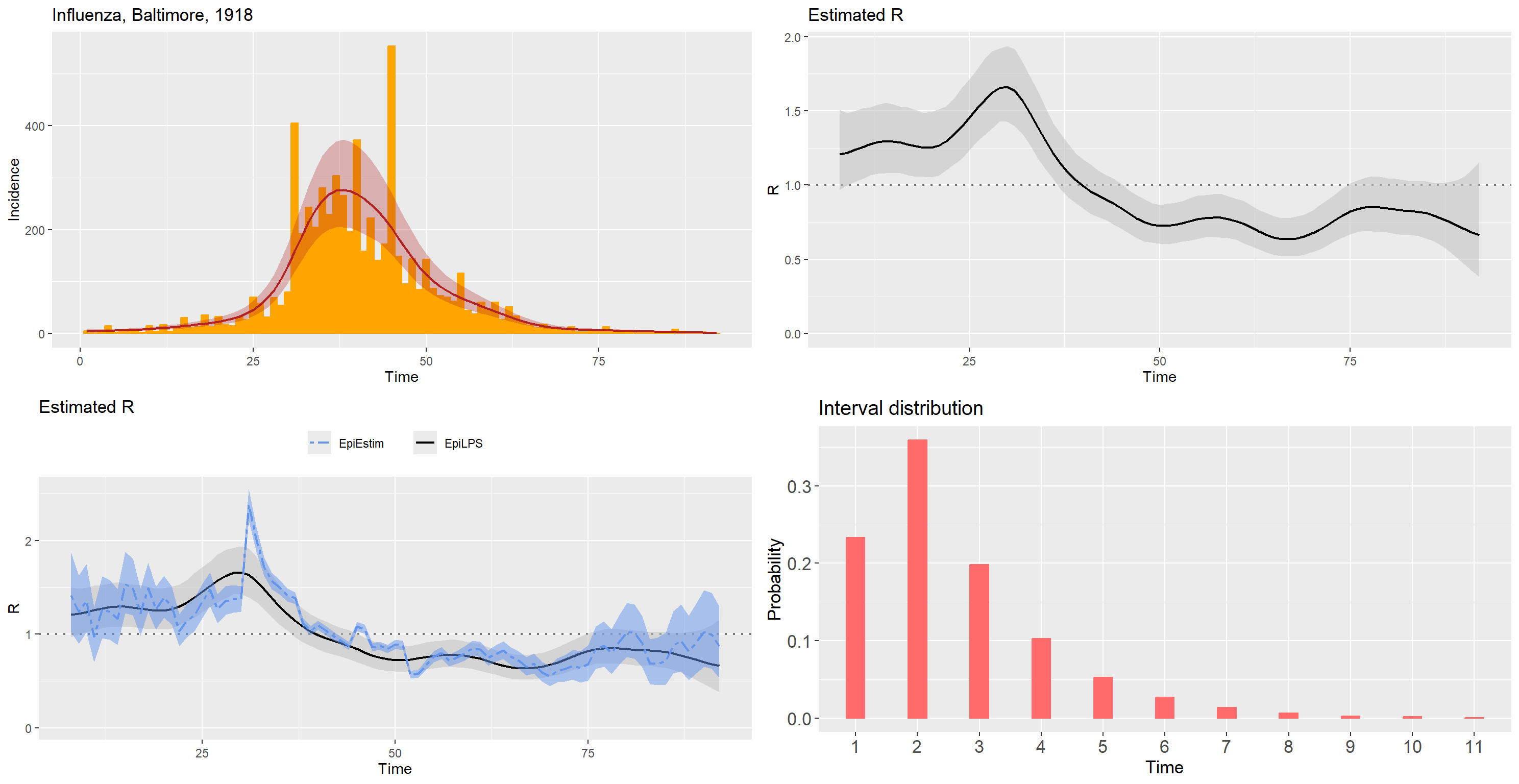

Data on the SARS epidemic in Hong Kong (2003)

data("SARS2003")
sarsDAT <- SARS2003
sars_incid <- sarsDAT$incidence
sars_si <- sarsDAT$si_distr[-1]
epifit_sars <- estimR(sars_incid, si = sars_si, CoriR = T)
epicurve_sars <- epicurve(sars_incid, datelab = "7d", title = "SARS, Hong Kong, 2003",
                         col = "ivory4", smooth = epifit_sars, smoothcol = "darkviolet")
Rplot_sars <- plot(epifit_sars, legendpos = "none")
Rplot_sars2 <- plot(epifit_sars, addfit = "Cori", legendpos = "top")
siplot_sars <- plot(Idist(probs = sars_si), barcol = "darkslateblue")
gridExtra::grid.arrange(epicurve_sars, Rplot_sars, Rplot_sars2, 
                        siplot_sars, nrow = 2, ncol = 2)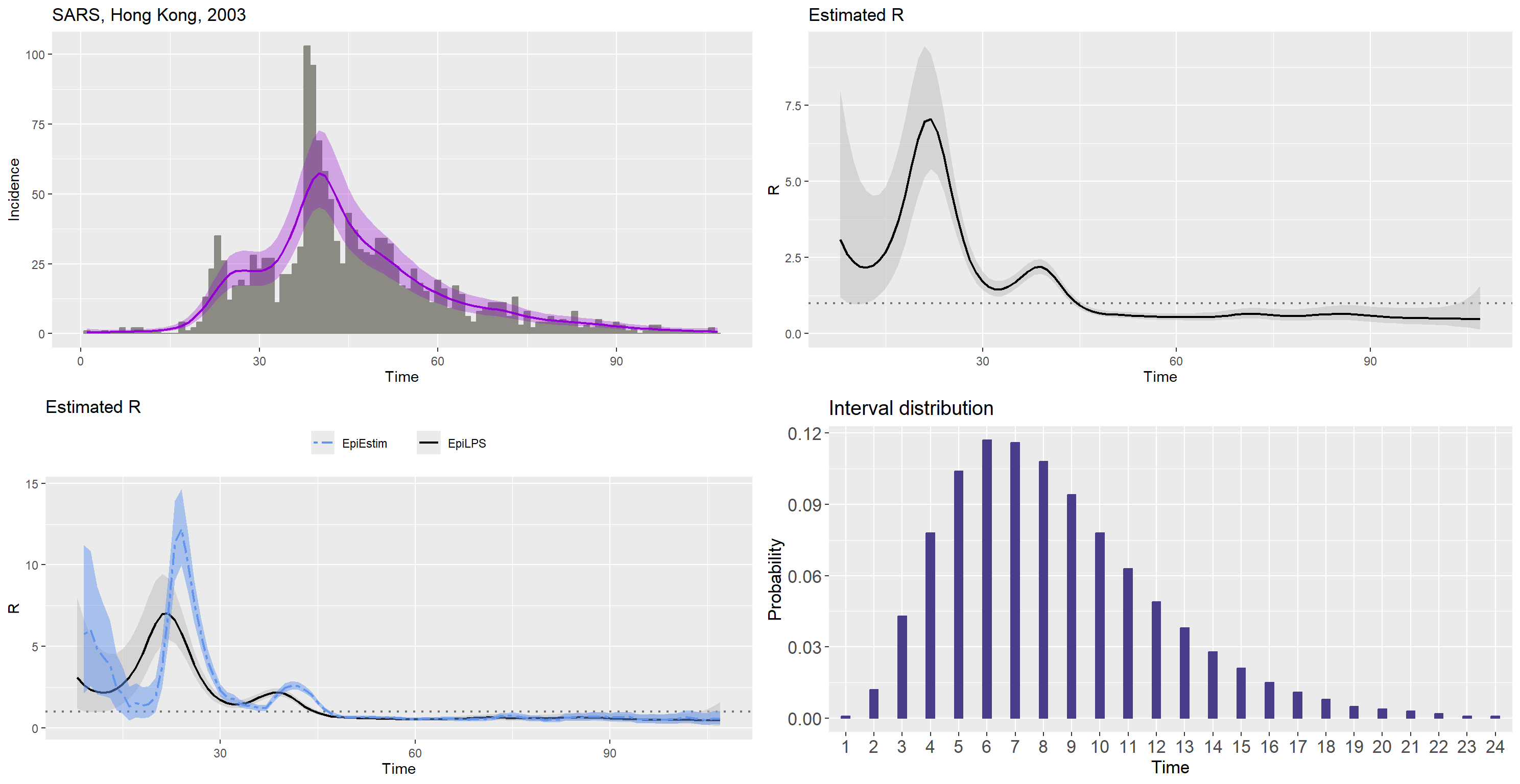

Funding

This project was funded by the European Union’s Research and Innovation Action under the H2020 work programme, EpiPose (grant number 101003688). It was also supported by the ESCAPE project (101095619) and the VERDI project (101045989), funded by the European Union. Views and opinions expressed are however those of the authors only and do not necessarily reflect those of the European Union or the Health and Digital Executive Agency (HADEA). Neither the European Union nor the granting authority can be held responsible for them.

References

Gressani, O., Wallinga, J., Althaus, C. L., Hens, N. and Faes, C. (2022). EpiLPS: A fast and flexible Bayesian tool for estimation of the time-varying reproduction number. PLoS Comput Biol 18(10): e1010618. https://doi.org/10.1371/journal.pcbi.1010618

Fraser C (2007) Estimating Individual and Household Reproduction Numbers in an Emerging Epidemic. PLoS ONE 2(8): e758. https://doi.org/10.1371/journal.pone.0000758

Cori, A., Ferguson, N.M., Fraser, C., Cauchemez, S. (2013) A new framework and software to estimate time-varying reproduction numbers during epidemics, American Journal of Epidemiology, 178(9), 1505–1512. https://doi.org/10.1093/aje/kwt133

Wallinga, J., & Teunis, P. (2004). Different epidemic curves for severe acute respiratory syndrome reveal similar impacts of control measures. American Journal of Epidemiology, 160(6), 509-516.