Nowcasting the reproduction number
by Bryan Sumalinab and Oswaldo Gressani
Motivation
The time-varying reproduction number \(\mathcal{R}_t\) (i.e., the average number of secondary cases generated by an infectious agent at time \(t\)) is a valuable parameter for quantifying the rate of infectious disease transmission and guiding public health responses during epidemics.
Daily incidence counts are classic data input streams in statistical
models for estimating \(\mathcal{R}_t\). The estimR()
and estimRmcmc() routines of EpiLPS simply require a
discrete serial interval distribution and a time series of incidence
data. The main advantage of the latter routines and the underlying
methodology is the simplicity with which they can be used as soon as
epidemic data streams in. For instance, with the daily number of
hospitalizations as an input, estimR() and
estimRmcmc() provide an estimate of \(\mathcal{R}_t\) based on a renewal equation
model that permits to rapidly grasp the big picture behind the
transmission dynamics of an infectious disease. An important factor that
is omitted in this modeling framework is the fact that daily incidence
counts are frequently subject to reporting delays. Various factors
contribute to these delays, for instance testing backlogs, overwhelmed
public health systems, communication and coordination challenges, and
issues in data collection and reporting processes. Such reporting delays
have a direct impact on \(\mathcal{R}_t\) estimates and may therefore
affect the timely assessment and response to an evolving epidemic.
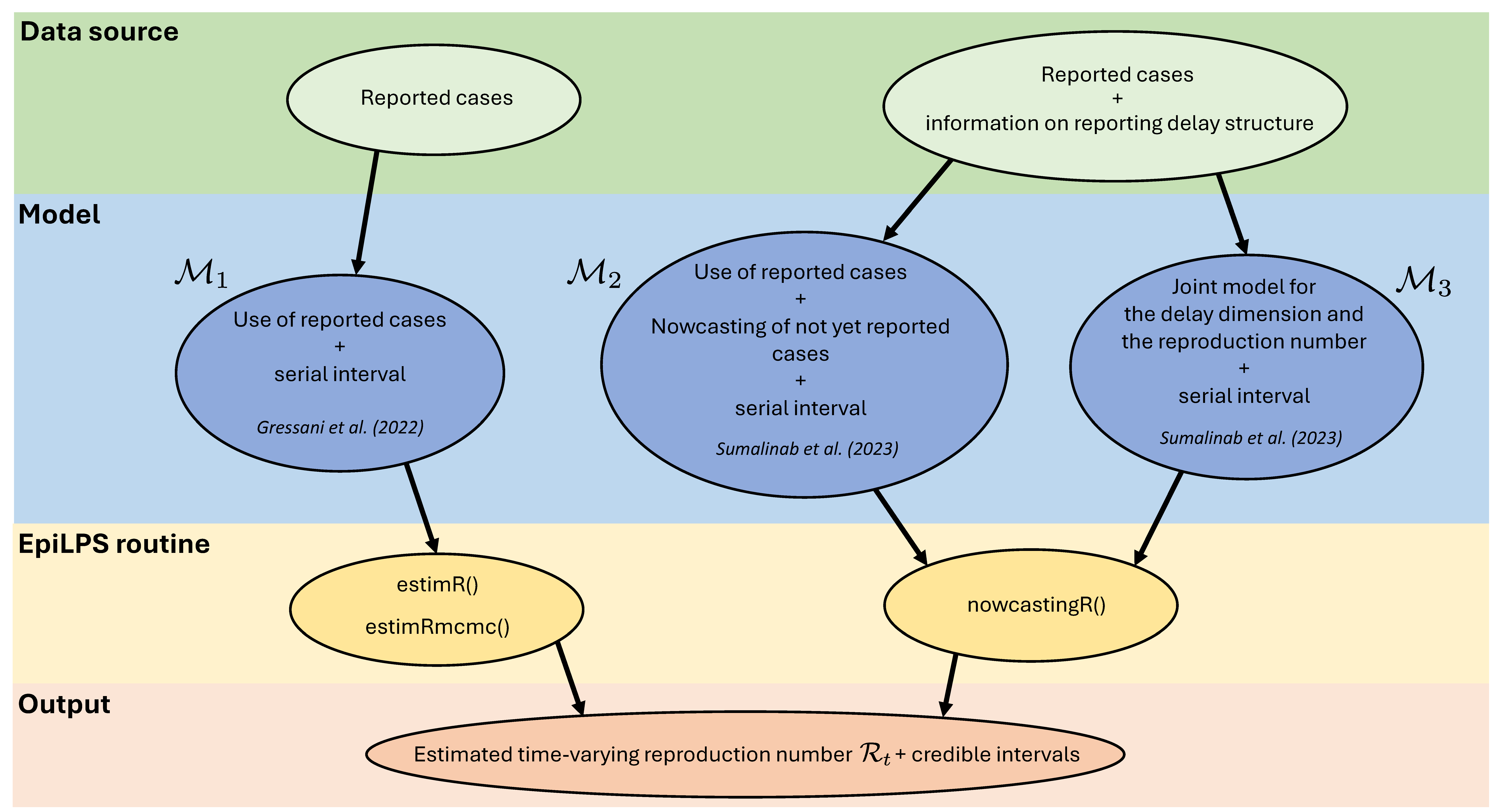
Sumalinab et al. (2024) address this delay issue by proposing a methodology to estimate \(\mathcal{R}_t\) that accounts for the impact of reporting delays through nowcasting. The paper compares three different models for estimating \(\mathcal{R}_t\) based on different data sources as illustrated in Figure 1. Model \(\mathcal{M}_1\) uses reported cases only (e.g. hospitalization data) without accounting for delays in reporting (https://epilps.com/Reproduction_number.html). Model \(\mathcal{M}_2\) uses reported cases and a nowcast of the not yet reported cases based on the methodology of Sumalinab et al. (2023). Finally, model \(\mathcal{M}_3\) uses a joint approach that simultaneously models the delay dimension and the time-varying reproduction number. The latter model is shown to deliver the most accurate estimates of the reproduction number in a simulation study.
The method evolves in the EpiLPS ecosystem, where Laplace
approximations and Bayesian P-splines form the core backbone for fast
and flexible inference. By integrating nowcasting within the \(\mathcal{R}_t\) estimation process, this
new methodology provides a more accurate reflection of the current
transmission dynamics. It also accounts for the uncertainty associated
with reporting delays, leading to a reliable quantification of
uncertainty as measured by Bayesian credible intervals. The
nowcastingR() function is now integrated in the EpiLPS
package and translates the methodology of Sumalinab et al. (2023) in a
simple and user-friendly routine. Before using
nowcastingR() to nowcast the reproduction number, it is
important to ensure that the data input for the nowcast is formatted
appropriately. Detailed guidelines, along with examples for the required
data input format can be found at https://epilps.com/Nowcasting.html.
Implementation
The code given below illustrates how to compute the nowcasted
reproduction number based on COVID-19 incidence data from Belgium in
2022 by using model \(\mathcal{M}_3\)
(the default). The dataset can be loaded from the EpiLPS package by
typing data("cov19incidence2022") and is already in the
desired format. Day of the week effects can be included in the model
with Monday serving as the default reference day. The discrete serial
interval distribution provided in Gressani et al. (2022) is used.
Sys.setlocale("LC_TIME", "English") # set locale language to English## [1] "English_United States.1252"data("cov19incidence2022") # load data
sicov19 <- c(0.344, 0.316, 0.168, 0.104, 0.068) # serial interval distribution
M3 <- nowcastingR(data = cov19incidence2022, si = sicov19, day.effect = TRUE)
knitr::kable(tail(M3$Rnow,10))| Time | status | R | Rsd | Rq0.025 | Rq0.05 | Rq0.25 | Rq0.50 | Rq0.75 | Rq0.95 | Rq0.975 | |
|---|---|---|---|---|---|---|---|---|---|---|---|
| 81 | 2022-03-22 | observed | 1.0152606 | 0.1094852 | 0.8233191 | 0.8515303 | 0.9446222 | 1.0152606 | 1.091181 | 1.210473 | 1.251950 |
| 82 | 2022-03-23 | observed | 1.0034625 | 0.1117456 | 0.8083014 | 0.8369017 | 0.9314883 | 1.0034625 | 1.080998 | 1.203172 | 1.245745 |
| 83 | 2022-03-24 | observed | 0.9908708 | 0.1161739 | 0.7892638 | 0.8186641 | 0.9162593 | 0.9908708 | 1.071558 | 1.199301 | 1.243976 |
| 84 | 2022-03-25 | observed | 0.9780289 | 0.1232272 | 0.7662050 | 0.7968710 | 0.8992308 | 0.9780289 | 1.063732 | 1.200371 | 1.248413 |
| 85 | 2022-03-26 | observed | 0.9660961 | 0.1375818 | 0.7338014 | 0.7669757 | 0.8788533 | 0.9660961 | 1.061999 | 1.216912 | 1.271927 |
| 86 | 2022-03-27 | nowcasted | 0.9557901 | 0.1558636 | 0.6985461 | 0.7346614 | 0.8580304 | 0.9557901 | 1.064688 | 1.243477 | 1.307766 |
| 87 | 2022-03-28 | nowcasted | 0.9468634 | 0.1821453 | 0.6558481 | 0.6957353 | 0.8344561 | 0.9468634 | 1.074413 | 1.288637 | 1.367009 |
| 88 | 2022-03-29 | nowcasted | 0.9388535 | 0.2124673 | 0.6119861 | 0.6555749 | 0.8102862 | 0.9388535 | 1.087821 | 1.344539 | 1.440304 |
| 89 | 2022-03-30 | nowcasted | 0.9317749 | 0.2465467 | 0.5683263 | 0.6153440 | 0.7859971 | 0.9317749 | 1.104590 | 1.410925 | 1.527651 |
| 90 | 2022-03-31 | nowcasted | 0.9260131 | 0.2826736 | 0.5276848 | 0.5776201 | 0.7630711 | 0.9260131 | 1.123749 | 1.484540 | 1.625024 |
Obtaining a summary of the resulting \(\mathcal{R}_t\) estimates during the final days of the epidemic is straightforward. In the status column, “nowcasted” indicates the days that have not yet reported cases as of the nowcast date. For this dataset, a maximum delay of five days was assumed. A plot of the estimated reproduction number can be obtained as follows:
plot(M3, nowcastcol = "orange", datelab = "15d")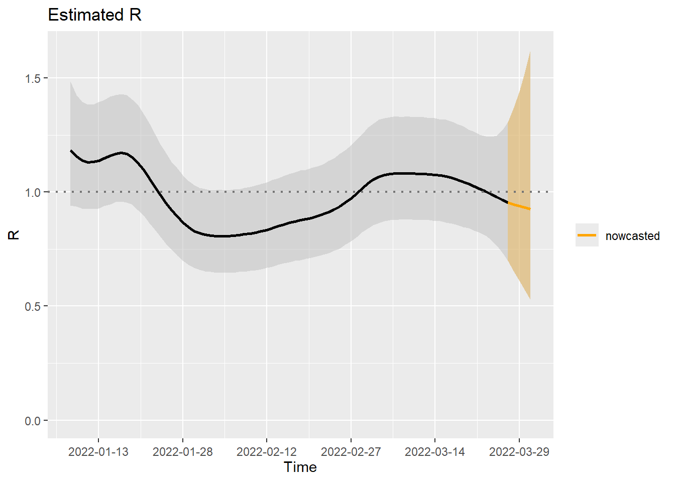
The colored part of the plot shows the nowcasted \(\mathcal{R}_t\) and its associated 95%
credible interval. An alternative method for estimating \(\mathcal{R}_t\) is by configuring the
method option to M2. Under the hood of this
approach, the reported cases and a nowcast of the not yet reported cases
are used as an input in the estimR() routine. While \(\mathcal{M}_2\) considers reporting delays,
it does not incorporate the associated uncertainty. This important
aspect has an impact on the estimated \(\mathcal{R}_t\) as illustrated below.
M2 <- nowcastingR(data = cov19incidence2022, si = sicov19, day.effect = TRUE, method = "M2")
plot(M2, nowcastcol = "cornflowerblue", datelab = "15d")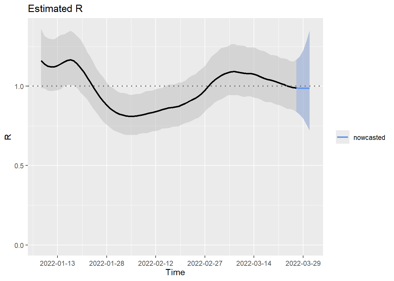
Model \(\mathcal{M}_1\) (i.e. making use of reported cases only) can be easily fitted as follows.
# Using reported cases only with estimR()
Rep_data <- cov19incidence2022[cov19incidence2022$Reported == "Reported", ]
y_rep <- aggregate(Cases ~ Date, data = Rep_data, sum)
M1 <- estimR(incidence = y_rep$Cases, si = sicov19)
Finally, we visualize the resulting \(\mathcal{R}_t\) point estimates of \(\mathcal{M}_1\), \(\mathcal{M}_2\) and \(\mathcal{M}_3\) respectively.
n <- nrow(M3$Rnow)
tstart <- 8
R_values <- c(M1$RLPS$R[tstart:n], M2$R$R[tstart:n], M3$Rnow$R[tstart:n])
Rmax <- max(R_values)
Rmin <- min(R_values)

data_R <- data.frame(Time = M3$Rnow$Time[tstart:n], M1R = M1$RLPS$R[tstart:n],
                     M2R = M2$R$R[tstart:n], M3R = M3$Rnow$R[tstart:n])

ggplot(data_R, aes(x = Time)) +
  geom_line(aes(y = M1R, color = "M1"), linewidth = 1) +
  geom_line(aes(y = M2R, color = "M2"), linetype = "dashed", linewidth = 1) +
  geom_line(aes(y = M3R, color = "M3"), linetype = "dotted", linewidth = 1) +
  labs(x = "Time", y = "R") +
  ylim(0, Rmax + 0.25) +
  scale_x_date(date_breaks = "15 days", date_labels = "%Y-%m-%d",
               limits = as.Date(c("2022-01-03", "2022-03-31"))) +
  geom_hline(yintercept = 1, linetype = "dotted",
             linewidth = 0.8, color = "gray46") +
  scale_color_manual(values = c("M1" = "black", "M2" = "blue", "M3" = "red")) +
  theme(legend.title = element_blank(), legend.position = "top",
    legend.justification = "center", legend.box = "horizontal") +
  geom_vline(xintercept = max(data_R$Time) - 5, lty = 2, linewidth = 0.8)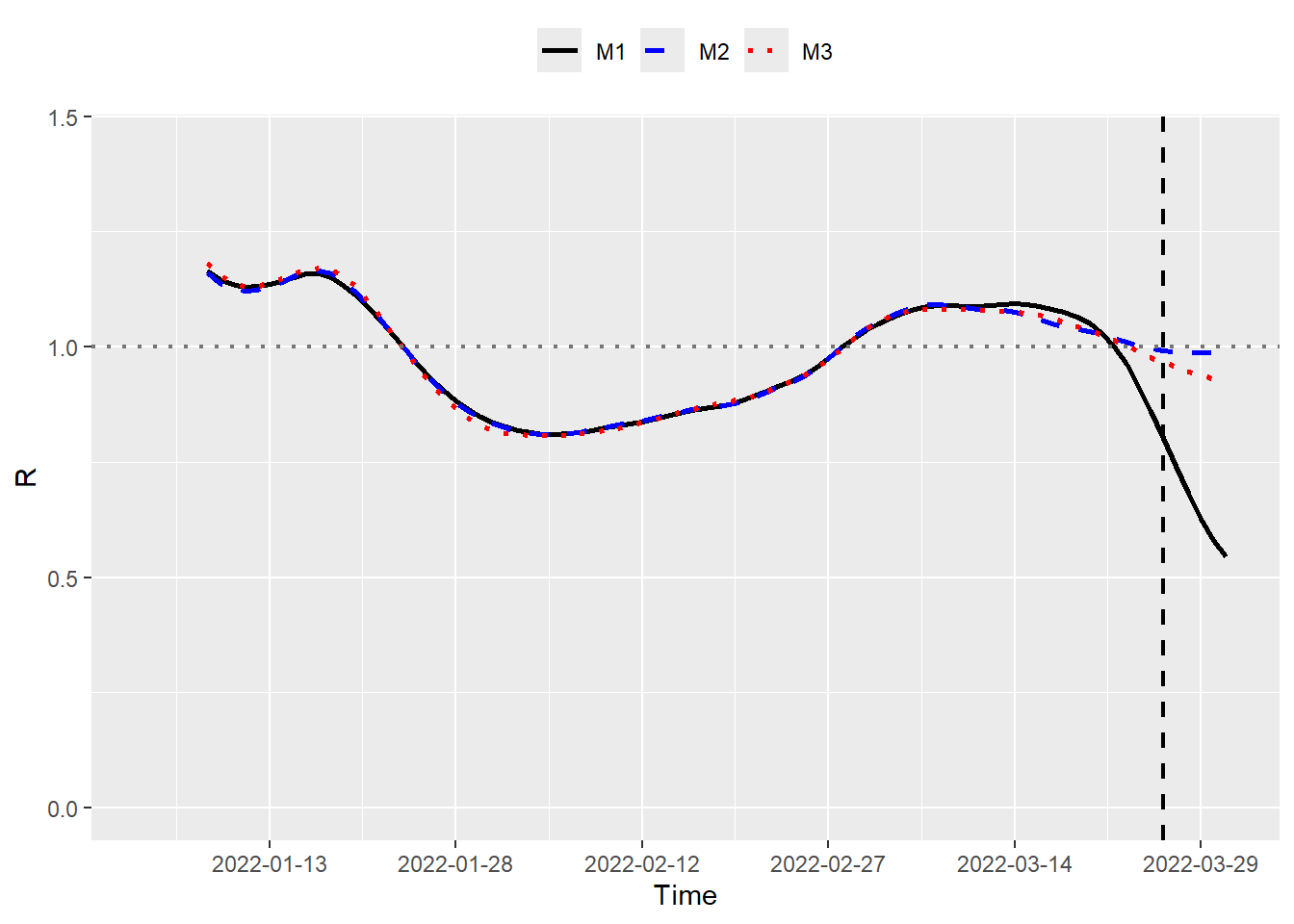
Dates located to the right of vertical dashed line (\(Time = 2022\text{-}03\text{-}26\)) represent calendar dates where cases have yet to be reported as of the current nowcast date. Consequently, there is not much difference in the \(\mathcal{R}_t\) estimates on the left side of the dashed line as we are using more or less the same amount of information for those dates. Furthermore, relying solely on reported cases (\(\mathcal{M}_1\)) leads to a downward bias in estimating \(\mathcal{R}_t\) (as expected), particularly on or around the nowcast date. Let us now compare the credible intervals of \(\mathcal{R}_t\) obtained with \(\mathcal{M}_2\) and \(\mathcal{M}_3\).
M2model <- M2$R[-c(1:tstart),]
M3model <- M3$R[-c(1:tstart),]
colnames(M2model) <- colnames(M3model)
combined_data <- rbind(M2model, M3model)

M2model$Model <- "M2"
M3model$Model <- "M3"
combined_data <- rbind(M2model, M3model)

ggplot(combined_data, aes(x = Time, y = R, color = Model)) +
  geom_line(linewidth = 1) +
  geom_ribbon(aes(ymin = Rq0.025, ymax = Rq0.975, fill = Model), alpha = 0.1) +
  labs(title = "Comparison of Rt estimates with 95% CI",
       x = "Time", y = "R") +
  ylim(0, max(M3$R[-c(1:tstart),][,"Rq0.975"])) +
  scale_x_date(date_breaks = "15 days", date_labels = "%Y-%m-%d",
                 limits = as.Date(c("2022-01-03", "2022-03-31"))) +
  geom_hline(yintercept = 1, linetype = "dotted",
             linewidth = 0.8, color = "gray46") +
  scale_color_manual(values = c("M2" = "blue", "M3" = "red")) +
  scale_fill_manual(values = c("M2" = "blue", "M3" = "red")) +
  theme_minimal() +
  theme(legend.title = element_blank())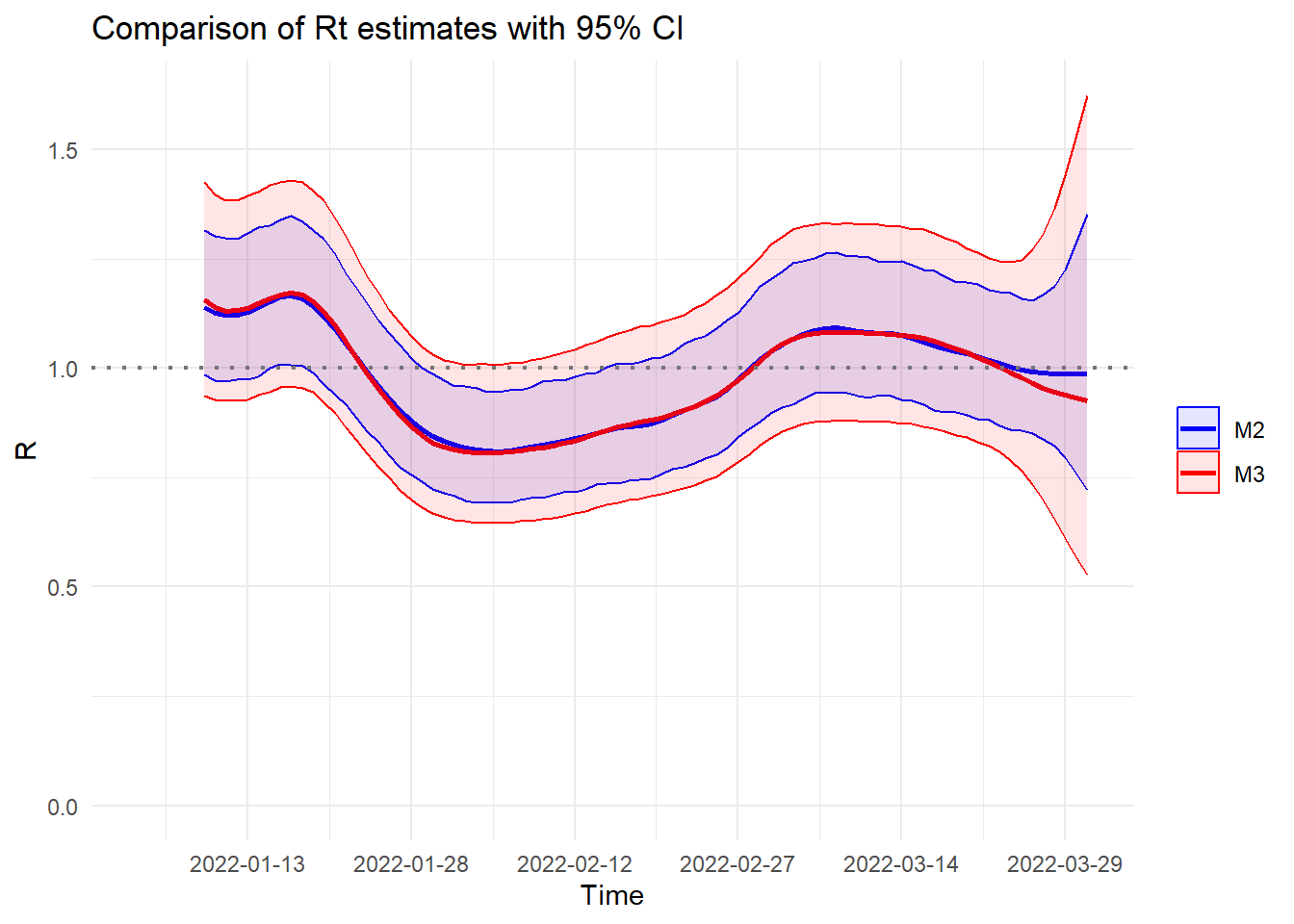
We only observe a minor difference in point estimates between the two models. However, model \(\mathcal{M}_3\) exhibits wider credible intervals due to the additional uncertainty coming from modeling the reporting delay dimension.
Funding
This work was supported by the ESCAPE project (101095619), co-funded by the European Union. Views and opinions expressed are however those of the authors only and do not necessarily reflect those of the European Union or European Health and Digital Executive Agency (HADEA). Neither the European Union nor the granting authority can be held responsible for them.
References
Sumalinab, B., Gressani, O., Hens, N. and Faes, C. (2024). An efficient approach to nowcasting the time-varying reproduction number. Epidemiology, 35(4):512-516. 10.1097/ede.0000000000001744
Sumalinab, B., Gressani, O., Hens, N. and Faes, C. (2024). Bayesian nowcasting with Laplacian-P-splines. Journal of Computational and Graphical Statistics (Accepted manuscript version). 10.1080/10618600.2024.2395414
Gressani, O., Wallinga, J., Althaus, C. L., Hens, N. and Faes, C. (2022). EpiLPS: A fast and flexible Bayesian tool for estimation of the time-varying reproduction number. PLoS Comput Biol 18(10): e1010618. https://doi.org/10.1371/journal.pcbi.1010618