Nowcasting
written by Bryan Sumalinab and edited by Oswaldo Gressani
Introduction
Nowcasting is a useful technique in epidemiology that addresses the problem of underreported cases caused by reporting delays. This approach uses statistical methods to predict (in real time) the number of cases that have not yet been reported. Reporting delays can be caused by administrative backlogs or slow data processing. By using nowcasting, health authorities can have a more accurate idea about the current spread of an infectious disease, enabling them to respond quickly to outbreaks and to efficiently allocate resources.
This documentation serves as a guide for implementing the nowcasting methodology developed by Sumalinab et al. (2023) within the EpiLPS package. The method is anchored around Laplacian-P-splines, a fundamental component of the EpiLPS framework. The idea behind the method is that the number of cases and reporting delays are modeled using two-dimensional penalized B-splines (P-splines) in a fully Bayesian framework. The nowcasted (predicted) not-yet-reported cases are then combined with the already reported cases to obtain an estimate of the actual number of cases at a given calendar time \(t\). Moreover, an estimate of the time-varying reporting delay distribution is also computed.
Simulated data
First, the nowcasting routine is illustrated through simulated data. Consider the following:
date.start <- as.Date('2023-01-01')         # start of the epidemic
date.now <- as.Date('2023-03-31')           # nowcast date
T.now <- as.numeric(format(date.now, "%j")) # numeric value for nowcast date
p <- c(0.25, 0.20, 0.15, 0.15, 0.15, 0.10)  # delay probabilities
max.delay <- length(p) - 1                  # maximum delay
overdisp <- 10                              # overdispersion parameter for simulated data
A function \(f(t)\) is chosen to represent the average epidemic curve for all cases, such that \(\mu(t) = \exp(f(t))\) for \(t = 1,...,T\):
f <- function(a1,a2,x) exp(a1 + a2*sin((2*pi*x)/250))
mu.sim <- f(a1  = 3, a2 = 1, x = 1:T.now)
Subsequently, for each time point \(t\), a random sample is generated denoted by \(y_t\), drawn from a negative binomial distribution with mean \(\mu(t)\) and fixed overdispersion parameter:
set.seed(0108)
simcases <- matrix(nrow = T.now,ncol = max.delay+1)
for (i in 1:T.now) {
  simcases[i,] <- rmultinom(n = 1, size = rnbinom(n = 1, mu = mu.sim[i], size = overdisp), prob = p)
}
dates <- seq(from = date.start,to = date.now,by = "day")
data <- data.frame(t = rep(1:T.now,times = max.delay+1),
                   d = rep(0:max.delay,each = T.now),
                   Cases = as.vector(simcases),
                   Date = rep(dates,times = max.delay+1))
data$Rep.date <- as.Date(data$Date) + data$d
The code provided above illustrates the generation of simulated data. Next, we differentiate between cases that have been reported and cases that have not yet been reported. All cases for which the sum of \(t\) and \(d\) is less than or equal to the nowcast date \(T.now\) will be categorized as “Reported”, otherwise “Not yet reported”.
Reported <- ifelse(data$t + data$d <= T.now, "Reported", "Not yet reported")
Reported <- factor(Reported, levels = c("Reported", "Not yet reported"))
data$Reported <- Reportedhead(data)## t d Cases Date Rep.date Reported
## 1 1 0 1 2023-01-01 2023-01-01 Reported
## 2 2 0 9 2023-01-02 2023-01-02 Reported
## 3 3 0 3 2023-01-03 2023-01-03 Reported
## 4 4 0 2 2023-01-04 2023-01-04 Reported
## 5 5 0 1 2023-01-05 2023-01-05 Reported
## 6 6 0 9 2023-01-06 2023-01-06 Reportedtail(data)## t d Cases Date Rep.date Reported
## 535 85 5 7 2023-03-26 2023-03-31 Reported
## 536 86 5 5 2023-03-27 2023-04-01 Not yet reported
## 537 87 5 2 2023-03-28 2023-04-02 Not yet reported
## 538 88 5 4 2023-03-29 2023-04-03 Not yet reported
## 539 89 5 1 2023-03-30 2023-04-04 Not yet reported
## 540 90 5 5 2023-03-31 2023-04-05 Not yet reportedThe above data frame contains the necessary data input for performing
a nowcast. The Date column represents the calendar date at
which cases were confirmed, the Rep.date column indicates
the reporting date, and the Cases column corresponds to the
number of cases associated with the respective Date and
Rep.date columns. The d column represents the
delay, and the t column is a numeric variable associated to
the calendar date. A plot of the simulated cases is given below:
sum_cases <- stats::aggregate(Cases ~ t, data, sum)
ggplot(data = sum_cases, aes(x = t, y = Cases)) + geom_bar(stat = "identity") +
  labs(x = "Time", y = "Simulated cases")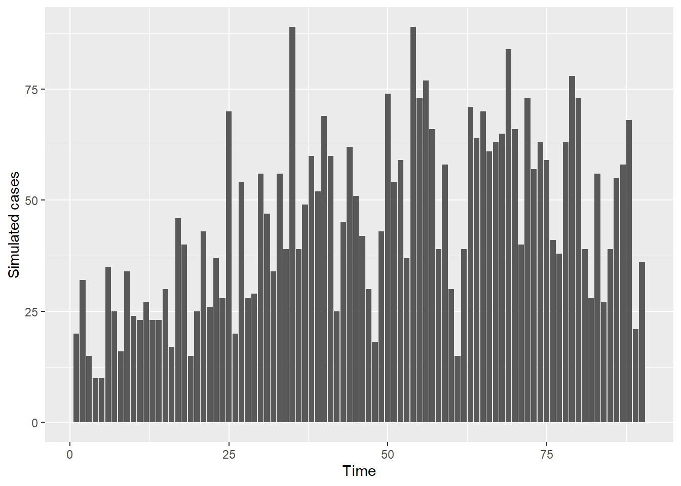
Next, the nowcasting() routine is implemented. To
exclude the day of the week effect, we set the day.effect
argument to FALSE.
# Nowcasting
nowcast <- nowcasting(data = data, day.effect = FALSE)
## Nowcast results:
## -------------------------------------------------------
## Time Date Nowcast CI95L CI95R
## 1 86 2023-03-27 54 50 61
## 2 87 2023-03-28 59 52 71
## 3 88 2023-03-29 61 50 84
## 4 89 2023-03-30 40 24 77
## 5 90 2023-03-31 52 32 102
## -------------------------------------------------------
## Time elapsed: 8sThe nowcasting results can be visualized using the code below:
plot(nowcast)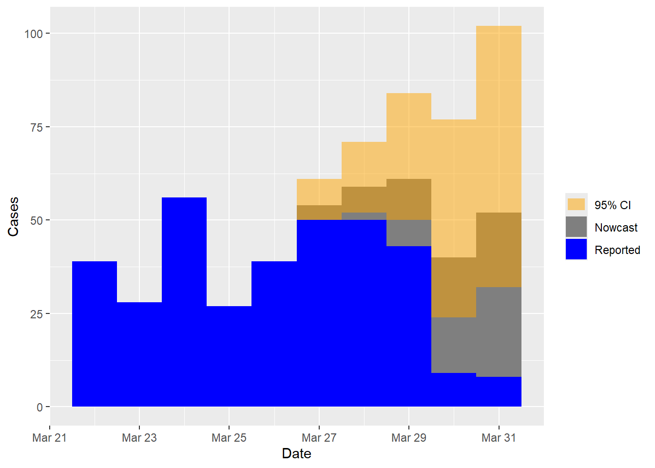
Note that the simulated data has a maximum delay of five days, meaning that for the most recent five days (from March 27 to March 31), there are cases that have not yet been reported. These dates involve nowcasting, as reflected in the nowcast plot above. In practice, our primary focus is on predicting the number of cases for the current nowcast day (March 31 in this example). Results of the nowcast can be examined as follows:
tail(nowcast$cases.now)## t y Date CI95L CI95R status
## 85 85 39 2023-03-26 NA NA observed
## 86 86 54 2023-03-27 50 61 nowcasted
## 87 87 59 2023-03-28 52 71 nowcasted
## 88 88 61 2023-03-29 50 84 nowcasted
## 89 89 40 2023-03-30 24 77 nowcasted
## 90 90 52 2023-03-31 32 102 nowcastedyindicates the number of nowcasted cases for each date, that is, reported + nowcasted.CI95LandCI95Rrepresent the lower and upper bound, respectively, of the 95% prediction interval.- The
statuscolumn indicates whether the calendar date involves nowcasting. - The last five rows in the output labeled as nowcasted in
the
statuscolumn are dates for which nowcasting is performed.
Since we are in presence of simulated data, we do have access to the number of cases that have not yet been reported. As such, we can compare the nowcasted results to the target values to evaluate the accuracy of the nowcasting process. The following code facilitates the visualization of this comparison:
data_CI <- na.omit(nowcast$cases.now)
levels(data$Reported) <- c("Reported", "Not yet reported", "Nowcast")
data <- data[data$Date > as.Date(max(data$Date)) - (2 * max(data$d)), ]
data1 <- aggregate(Cases ~ Date + Reported, data, sum)

ggplot(data = data1, aes(x = Date, y = Cases, fill = Reported)) +
    geom_col(width = 1, position = position_stack(reverse = TRUE)) +
    geom_step(data = data_CI, aes(x = Date + 0.5, y = y), colour = "red", linewidth = 0.8,
              direction = "vh", inherit.aes = FALSE) +
    scale_fill_manual(values = c("blue", "grey50", "red"),
                      name = "", drop = FALSE) +
    geom_crossbar(data = data_CI, aes(x = Date, y = y, ymin = CI95L, ymax = CI95R),
                  fill = adjustcolor("orange", alpha = 0.3),
                  colour = NA, width = 1, inherit.aes = FALSE)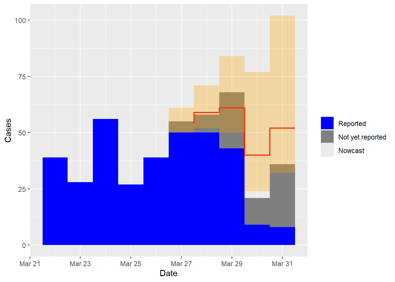
The plot above shows the reported cases in blue and the not yet reported cases in grey. The red line represents the nowcast that combines both reported and predicted cases. The orange shading represents the 95% prediction interval.
Mortality data (Belgium)
Now, the nowcasting routine is applied to the COVID-19 mortality data in Belgium for the year 2021. The unaggregated historical data (mortality and incidence cases) can be found on the Sciensano research institute website, accessible at https://epistat.sciensano.be/covid/. For illustration purposes, we use data from the initial three months (January through March 2021) with the following columns:
- Date - date on which a patient died from COVID-19.
- Rep.date - date on which the COVID-19 death was reported.
- Cases : number of COVID-19 deaths.
load("data/mortality2021raw.RData")
head(mort2021raw)
tail(mort2021raw)
Preparing the data for nowcasting
The raw dataset has to be transformed to be in a suitable format. In
particular, three additional columns must be added: t,
d, and Reported as explained below:
- Create a new column
tas a numeric variable forDate, ranging from 1 to \(T\), where \(T\) is the nowcast date and maximum value in theDatecolumn. - Create a new column
das a numeric value for the delay, ranging from 1 to \(D\), where \(D\) is the maximum delay. This is simply the difference betweenRep.dateandDatefor all rows. - Create a new column
Reportedas a factor with two labels: Reported and Not yet reported. For each row, determine whethert+dis less than or equal to \(T\). If it is, label the row as Reported; otherwise, label it as Not yet reported. - Ensure that all combinations of
tanddfrom 1 to \(T\) and 1 to \(D\) are represented in the dataset. For those combinations where there are no cases, set theCasescolumn to 0. By following these steps, we obtain a dataset that is appropriately formatted for the nowcasting routine.
date.start <- min(mort2021raw$Date)

# Calculate 't' as the numeric column for Date
mort2021raw$t <- as.integer(mort2021raw$Date - date.start + 1)
# Calculate 'd' as the numeric difference between 'Rep.date' and 'Date'
mort2021raw$d <- as.numeric(mort2021raw$Rep.date - mort2021raw$Date)

date.now <- as.Date("2021-03-31") # set nowcast date
T.now <- as.numeric(date.now - date.start) + 1 # numeric value for the nowcast date
max.delay <- as.numeric(max(mort2021raw$Rep.date - mort2021raw$Date)) # maximum delay
expand <- expand.grid("t" = 1:T.now,"d" = 0:max.delay) # create t,d combinations

# Merge the data frames 'mort2021raw' and 'expand' using merge
mort_data <- merge(mort2021raw, expand, by = c("t", "d"), all = TRUE)
# Calculate 'Date' as the minimum 'Date' from 'mort2021raw' plus 't' minus 1
mort_data$Date <- as.Date(min(mort2021raw$Date) + mort_data$t - 1)
# Calculate 'Rep.date' as 'Date' + 'd'
mort_data$Rep.date <- mort_data$Date + mort_data$d
# Replace negative or NA 'Cases' with 0
mort_data$Cases <- ifelse(is.na(mort_data$Cases) | mort_data$Cases < 0, 0, mort_data$Cases)
# Arrange the data by 'd'
mort_data <- mort_data[order(mort_data$d), ]

#### Label the cases satisfying t + d <= T as 'Reported', else 'Not yet reported'.
Reported <- ifelse(mort_data$t + mort_data$d <= T.now, "Reported", "Not yet reported")
Reported <- factor(Reported, levels = c("Reported", "Not yet reported"))
mort_data$Reported <- Reported
rownames(mort_data) <- NULL
Overview of the input mortality data
head(mort_data)## t d Date Rep.date Cases Reported
## 1 1 0 2020-12-31 2020-12-31 0 Reported
## 2 2 0 2021-01-01 2021-01-01 0 Reported
## 3 3 0 2021-01-02 2021-01-02 0 Reported
## 4 4 0 2021-01-03 2021-01-03 0 Reported
## 5 5 0 2021-01-04 2021-01-04 0 Reported
## 6 6 0 2021-01-05 2021-01-05 0 ReportedNowcasting
Next, we perform the nowcasting using the formated mortality data. The model will include the day-of-the-week effect as a default. Additionally, we configure the R language setting to English, since days of the week are specified in English.
Sys.setlocale("LC_TIME", "English") # Set language to English## [1] "English_United States.1252"nowcast.mort <- nowcasting(data = mort_data) # Nowcasting## Nowcast results:
## -------------------------------------------------------
## Time Date Nowcast CI95L CI95R
## 1 87 2021-03-27 28 27 29
## 2 88 2021-03-28 24 23 28
## 3 89 2021-03-29 34 31 43
## 4 90 2021-03-30 22 9 67
## 5 91 2021-03-31 19 5 64
## -------------------------------------------------------
## Time elapsed: 5.76splot(nowcast.mort) # Nowcast plot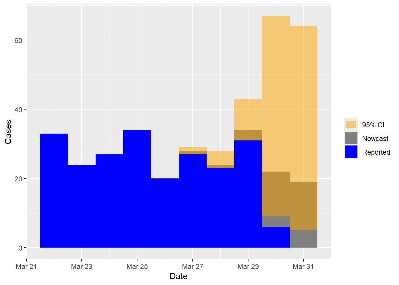
The estimated delay distribution can be obtained as follows:
plot(nowcast.mort, type = "delay")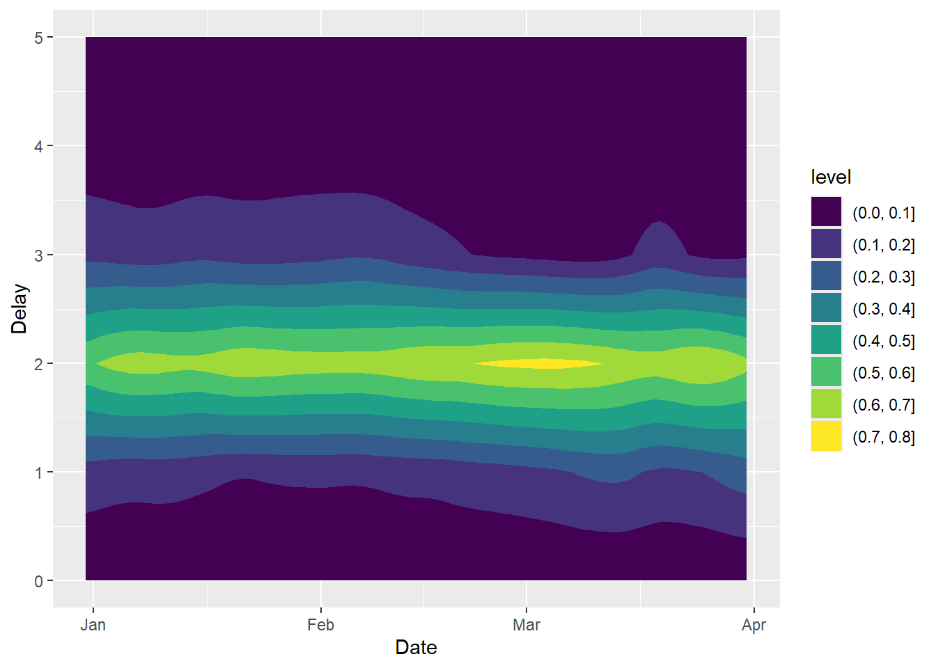
The above plot suggests that most cases are typically reported with a two-day delay. The code below can be used to obtain a three-dimensional plot of the smoothed surface on the time and delay dimension (This code only works with the GitHub version of EpiLPS 1.4.0 for the moment).
mint <- min(nowcast.mort$data$t)
maxt <- max(nowcast.mort$data$t)
mind <- min(nowcast.mort$data$d)
maxd <- max(nowcast.mort$data$d)
Kt <- nowcast.mort$Kt
Kd <- nowcast.mort$Kd
xi_mode <- nowcast.mort$xi_mode

# Fine grid for time and delay
tfine <- seq(mint, maxt, length.out = 100)
dfine <- seq(mind, maxd, length.out = 50)

# B-spline basis matrix
Btfine <- EpiLPS:::Rcpp_KercubicBspline(tfine, lower = mint, upper = maxt, K = Kt)
Bdfine <- EpiLPS:::Rcpp_KercubicBspline(dfine, lower = mind, upper = maxd, K = Kd)
Bfine <- kronecker(Bdfine, Btfine)

# Estimated smooth surface
mufine <- exp(Bfine %*% xi_mode[1:(Kt * Kd)])
Zfine <- matrix(mufine, nrow = length(tfine), ncol = length(dfine))

# Plot
par(mfrow = c(2,1))
persp3D(tfine, dfine, Zfine, theta = 140, phi = 15,
        expand = 0.5, shade = 0.10, zlab = "", xlab = "Time",
        ylab ="Delay", ticktype = "detailed", colkey = FALSE)
persp3D(tfine, dfine, Zfine, theta = 60, phi = 20,
        expand = 0.5, shade = 0.10, zlab = "", xlab = "Time",
        ylab ="Delay", ticktype = "detailed", colkey = FALSE)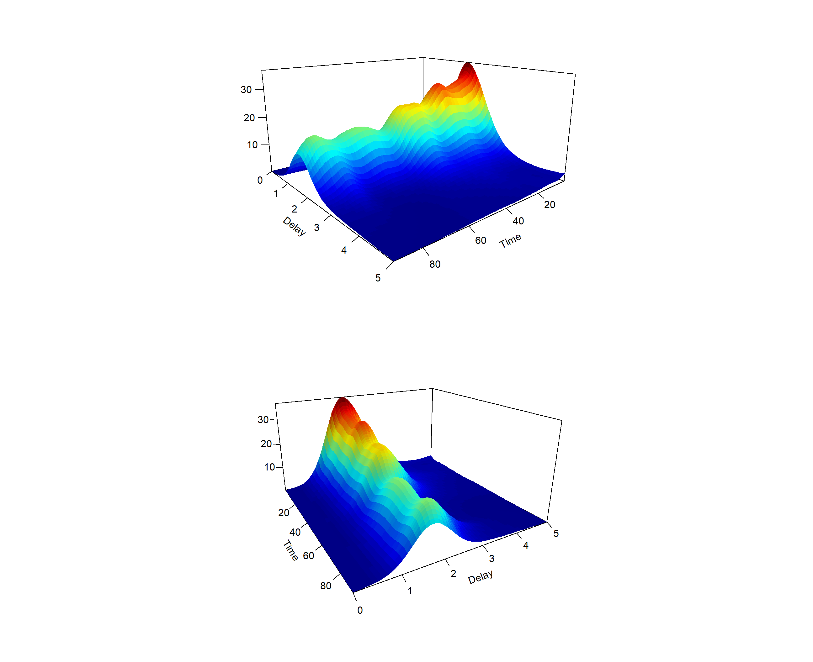
# Nowcast result
tail(nowcast.mort$cases.now)
## t y Date CI95L CI95R status
## 86 86 20 2021-03-26 NA NA observed
## 87 87 28 2021-03-27 27 29 nowcasted
## 88 88 24 2021-03-28 23 28 nowcasted
## 89 89 34 2021-03-29 31 43 nowcasted
## 90 90 22 2021-03-30 9 67 nowcasted
## 91 91 19 2021-03-31 5 64 nowcastedIncidence data (Belgium)
This example uses COVID-19 incidence data in Belgium for the year
2022. The data has a maximum delay of five days and has already been
transformed into a suitable format for the nowcasting()
routine.
# COVID-19 incidence data in Belgium
data("cov19incidence2022")
incidence2022 <- cov19incidence2022
head(incidence2022)
## t d Date Rep.date Cases Reported
## 1 1 0 2022-01-01 2022-01-01 0 Reported
## 2 2 0 2022-01-02 2022-01-02 0 Reported
## 3 3 0 2022-01-03 2022-01-03 0 Reported
## 4 4 0 2022-01-04 2022-01-04 0 Reported
## 5 5 0 2022-01-05 2022-01-05 0 Reported
## 6 6 0 2022-01-06 2022-01-06 0 Reportedtail(incidence2022)## t d Date Rep.date Cases Reported
## 535 85 5 2022-03-26 2022-03-31 6 Reported
## 536 86 5 2022-03-27 2022-04-01 7 Not yet reported
## 537 87 5 2022-03-28 2022-04-02 75 Not yet reported
## 538 88 5 2022-03-29 2022-04-03 7 Not yet reported
## 539 89 5 2022-03-30 2022-04-04 1 Not yet reported
## 540 90 5 2022-03-31 2022-04-05 4 Not yet reported# Nowcasting
nowcast.inc <- nowcasting(data = incidence2022)## Nowcast results:
## -------------------------------------------------------
## Time Date Nowcast CI95L CI95R
## 1 86 2022-03-27 3614 3604 3643
## 2 87 2022-03-28 17670 17580 17976
## 3 88 2022-03-29 12917 9208 22840
## 4 89 2022-03-30 10603 3021 29651
## 5 90 2022-03-31 8909 2328 29453
## -------------------------------------------------------
## Time elapsed: 8.09splot(nowcast.inc)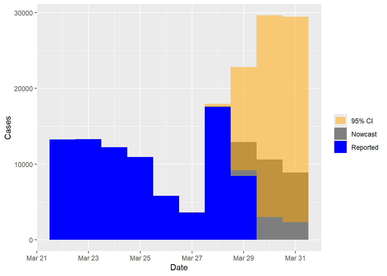
tail(nowcast.inc$cases.now)## t y Date CI95L CI95R status
## 85 85 5829 2022-03-26 NA NA observed
## 86 86 3614 2022-03-27 3604 3643 nowcasted
## 87 87 17670 2022-03-28 17580 17976 nowcasted
## 88 88 12917 2022-03-29 9208 22840 nowcasted
## 89 89 10603 2022-03-30 3021 29651 nowcasted
## 90 90 8909 2022-03-31 2328 29453 nowcastedThe prediction interval for the incidence data is significantly wider due to the unstable nature of this dataset. There are several sources of uncertainty, such as no reported cases on the nowcast day, almost no cases reported with one-day delays, numerous zeros and a wide range of case counts from zero to thousands. All these factors contribute to a significant level of uncertainty in the predictions.
Funding
This project was funded by the European Union Research and Innovation Action under the H2020 work programme EpiPose (grant number 101003688).
References
Gressani, O., Wallinga, J., Althaus, C. L., Hens, N. and Faes, C. (2022). EpiLPS: A fast and flexible Bayesian tool for estimation of the time-varying reproduction number. PLoS Comput Biol 18(10): e1010618. https://doi.org/10.1371/journal.pcbi.1010618
Sumalinab, B., Gressani, O., Hens, N. and Faes, C. (2024). Bayesian nowcasting with Laplacian-P-splines. Journal of Computational and Graphical Statistics (Accepted manuscript version). 10.1080/10618600.2024.2395414