Estimation of incubation times
written by Oswaldo Gressani
Introduction
The EpiLPS (Epidemiological modeling with Laplacian-P-Splines) package can be used to estimate the incubation period of an infectious disease (the time elapsed between infection and symptom onset) following the methodology of Gressani et al. (2023). A challenge one typically encounters when attempting to model the incubation period is the imperfect information that accompanies infection times. The latter are rarely observed in practice and are usually only known to lie within a time window (often called exposure interval). Together with symptom onset times (which are more easily observed and thus available), exposure intervals can be used in a statistical modeling framework to construct an estimate of the incubation period.
EpiLPS proposes a Bayesian framework to estimate the distribution of the incubation period based on coarse data, i.e. data that has an interval-censored flavor as described above for the exposure window. A semi-parametric model involving Laplace approximations and penalized B-splines is used to estimate the incubation period distribution. The posterior distribution of the model parameters is sampled by means of a Metropolis-adjusted Langevin algorithm that is embedded in a Gibbsian scheme. Time consuming subroutines are coded in C++ and integrated in R via the Rcpp package so that computational time is relatively low. The semi-parametric incubation fit is then used to inform a set of distributions belonging to well-known parametric families that are often used to model incubation times and the Bayesian information criterion guides towards the ‘best’ fit. As such, the methodology provides an interesting alternative to classic Bayesian approaches that solely rely on purely parametric models. This preprint gives a detailed description of the methodology and explains how it is naturally nested within the EpiLPS framework.
The estimIncub() (estimation of incubation period)
routine is the key function that allows the user to compute an estimate
of the incubation density based on three main inputs:
x: A data frame containing the lower and upper bound of the incubation interval.K: An integer specifying the number of B-splines to smooth the incubation density.niter: The number of MCMC samples required.
The data frame x has two columns. The first column
should correspond to the lower bound of the incubation interval and the
second column to the upper bound. From (observed) symptom onset times
\(t^{\mathcal{S}}\) and exposure
intervals \(\mathcal{E}=[t^{E_L},t^{E_R}]\), incubation
intervals \(\mathcal{I}=[t^{\mathcal{I}_L},
t^{\mathcal{I}_R}]\) can be easily constructed with lower bound
\(t^{\mathcal{I}_L}=t^{\mathcal{S}}-t^{E_R}\)
and upper bound \(t^{\mathcal{I}_R}=t^{\mathcal{S}}-t^{E_L}\).
The number of B-splines basis functions is by default set to
K=10 but more can be added if required. Finally, the number
of MCMC iterations is by default set to niter=1000.
Simulated example
A simulated example is first used to illustrate the
estimIncub() routine, where symptom onset times and
infecting exposure windows are generated by means of the
incubsim() routine. The latter function allows to generate
a sample of symptom onset times and exposure windows for a desired
sample of size \(n\) with a Data
Generating Mechanism (DGM) that allows for different distributions of
the incubation period, namely a LogNormal, Weibull, a two-component
mixture of Weibulls and a Gamma distribution. Below is the code for
generating a sample of size \(n=200\)
with a Weibull incubation density. The option coarseness is
set to two days (this will on average set the exposure interval width of
the generated data to two days). With $Dobsincub the user
is able to access the lower and upper bound of the incubation interval
(which will be the x input in estimIncub()).
Here, the generated incubation windows (in days) for the first five
individuals are shown.
set.seed(123)
simdat <- incubsim(incubdist = "Weibull", n = 100, coarseness = 2)
knitr::kable(head(simdat$Dobsincub, 5))| tL | tR |
|---|---|
| 3.140144 | 4.854940 |
| 4.591608 | 6.388431 |
| 3.207375 | 4.898248 |
| 8.411519 | 11.502474 |
| 6.906292 | 9.660761 |
The true incubation distribution in the above DGM is a Weibull with a
mean of 6.4 days and a standard deviation of 2.3 days (Backer et
al. 2020). Detailed information on the DGM can be found by typing
?incubsim() in the R console. The estimIncub()
routine is now applied on the above generated dataset.
fitsim <- estimIncub(x = simdat$Dobsincub, verbose = TRUE, tmax = 20)## ----------------------------------------------------------------
## Time elapsed: 3.21 seconds.
## Fitted density is Weibull with shape=2.811 and scale=7.408.
## Mean incubation period (days): 6.597 with 95% CI: 6.372-6.836.
## 95th percentile (days): 10.945 with 95% CI: 10.62-11.465.
## ----------------------------------------------------------------Typing fitsim$stats gives access to point estimates (and
credible intervals) for crucial features of the incubation distribution
(Mean, SD, quantiles).
knitr::kable(head(fitsim$stats))| PE | CI90L | CI90R | CI95L | CI95R | |
|---|---|---|---|---|---|
| Mean | 6.597295 | 6.412497 | 6.836487 | 6.371662 | 6.836487 |
| SD | 2.541933 | 2.418050 | 2.693500 | 2.401534 | 2.693500 |
| q0.05 | 2.574895 | 2.385706 | 2.807828 | 2.360121 | 2.874251 |
| q0.1 | 3.326458 | 3.125690 | 3.566497 | 3.093982 | 3.637859 |
| q0.15 | 3.881047 | 3.674159 | 4.125784 | 3.643898 | 4.184041 |
| q0.2 | 4.344429 | 4.135072 | 4.584816 | 4.100857 | 4.635539 |
The fitted incubation density (in red) can also be graphically
compared with the target Weibull density (in black) by accessing the
different elements of the fitsim object.
plot(fitsim$tg, fitsim$ftg, col = "royalblue", type = "l", lwd = 2, xlab = "Time (in days)",
     ylab = "Probability density function", ylim = c(0,0.16))
lines(simdat$tdom, dweibull(simdat$tdom, shape = 3.00060, scale = 7.170345),
      type = "l", lwd = 2)
legend("topright", c("Target", "Estimation"), col = c("black","royalblue"), lwd = c(2,2), bty = "n")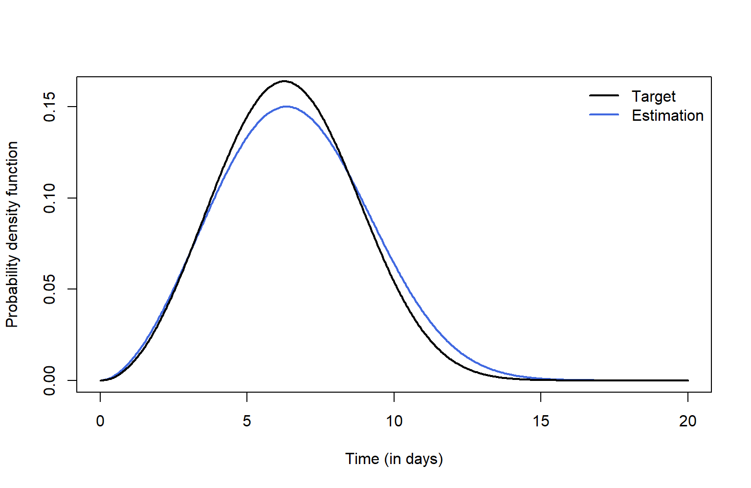
The plot() function can also directly be applied to the
fitsim object to obtain the fitted probability density
function and (if required) a bar plot showing the incubation windows.
The gray shaded area corresponds to the \(95\%\) credible interval.
gridExtra::grid.arrange(plot(fitsim, typ = "incubwin"), plot(fitsim, type = "pdf"),
                        nrow = 1, ncol = 2)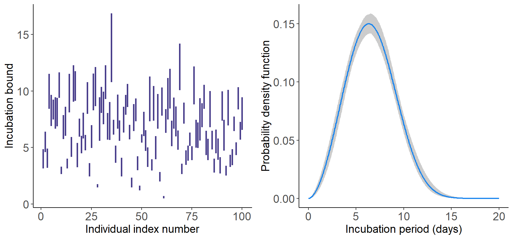
Real data example
As a real data application, we consider the dataset on MERS-CoV infections in South Korea downloaded from Virlogeux et al. (2016) https://wwwnc.cdc.gov/eid/article/22/3/15-1437_article. The dataset contains lower and upper bounds of the incubation period (in days) for 109 patients and information on the death status (0-alive; 1-dead). First, we read the data and transform the discrete daily values into continuous values by adding a uniformly distributed random noise.
# Read data
data <- read.csv(file = "data/Korea_MERS2015.csv", header = TRUE, skip = 1)
data_exposure <- data[data$missing_exposure == 0, ] # Skip missing exposure dates

set.seed(123)
Dobs <- data.frame(tL = data_exposure$IncP_min, tR = data_exposure$IncP_max)
Dobs <- Dobs[-which(Dobs$tR > 20),] # Remove (two) "outliers".
n <- nrow(Dobs)
for(i in 1:n) {
  u1 <- runif(1)
  Dobs$tL[i] <- Dobs$tL[i] + u1
  u2 <- runif(1)
  while (u2 <= u1) u2 <- runif(1)
  Dobs$tR[i] <- Dobs$tR[i] + u2
}
The lower and upper incubation bounds for the first five patients are shown below.
knitr::kable(head(Dobs, 5))| tL | tR |
|---|---|
| 0.2875775 | 15.788305 |
| 4.4089769 | 4.883017 |
| 9.9404673 | 9.956833 |
| 8.4533342 | 8.677571 |
| 7.5726334 | 9.899825 |
Next, we use the estimIncub() routine with
K=15 B-splines and niter=5000 MCMC iterations
and plot the estimated incubation distribution together with the
incubation bounds. EpiLPS selects a Weibull fit to the data with a mean
incubation period of 7.4 days (95% CI 7.1-7.7 days).
incubfit <- estimIncub(x = Dobs, K = 15, niter = 5000, verbose = TRUE, tmax = 20)## ----------------------------------------------------------------
## Time elapsed: 17.57 seconds.
## Fitted density is Weibull with shape=2.727 and scale=8.308.
## Mean incubation period (days): 7.391 with 95% CI: 7.129-7.658.
## 95th percentile (days): 12.424 with 95% CI: 12.013-12.978.
## ----------------------------------------------------------------gridExtra::grid.arrange(plot(incubfit, type = "incubwin"), plot(incubfit, type = "pdf"), nrow = 1, ncol = 2)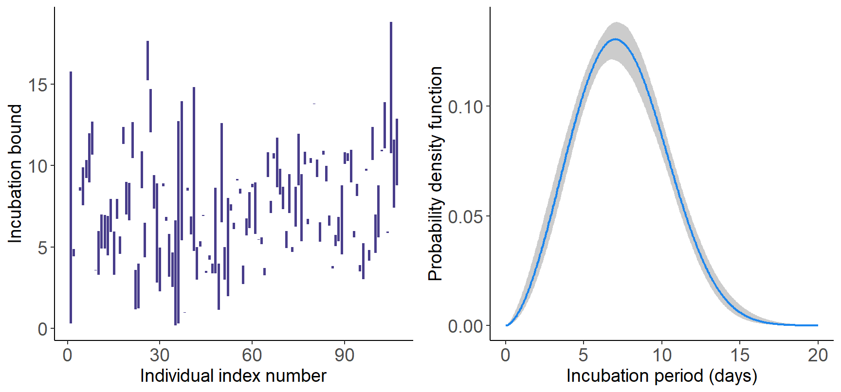
As we also have information on whether a patient is dead or alive, we can stratify our analysis by death status and compare the estimated incubation distribution of those who survived and those who died from MERS-CoV infection.
set.seed(123)
Dobs2 <- data.frame(tL = data_exposure$IncP_min, tR = data_exposure$IncP_max,
                   surv = data_exposure$Death_status)
Dobs2 <- Dobs2[-which(Dobs2$tR > 20),]
Dobs_surv <- Dobs2[Dobs2$surv == 0,][1:2]
nsurv <- nrow(Dobs_surv)
Dobs_dead <- Dobs2[Dobs2$surv == 1,][1:2]
ndead <- nrow(Dobs_dead)

set.seed(123)
for(i in 1:nsurv) {
  u1 <- runif(1)
  Dobs_surv$tL[i] <- Dobs_surv$tL[i] + u1
  u2 <- runif(1)
  while (u2 <= u1) u2 <- runif(1)
  Dobs_surv$tR[i] <- Dobs_surv$tR[i] + u2
}

for(i in 1:ndead) {
  u1 <- runif(1)
  Dobs_dead$tL[i] <- Dobs_dead$tL[i] + u1
  u2 <- runif(1)
  while (u2 <= u1) u2 <- runif(1)
  Dobs_dead$tR[i] <- Dobs_dead$tR[i] + u2
}
incub_surv <- estimIncub(x = Dobs_surv, K = 15, niter = 5000, verbose = TRUE, tmax = 20)## ----------------------------------------------------------------
## Time elapsed: 26.56 seconds.
## Fitted density is Weibull with shape=2.856 and scale=8.575.
## Mean incubation period (days): 7.641 with 95% CI: 7.322-7.933.
## 95th percentile (days): 12.591 with 95% CI: 12.121-13.191.
## ----------------------------------------------------------------incub_dead <- estimIncub(x = Dobs_dead, K = 15, niter = 5000, verbose = TRUE, tmax = 20)## ----------------------------------------------------------------
## Time elapsed: 15.41 seconds.
## Fitted density is Gamma with shape=5.35 and rate=0.811.
## Mean incubation period (days): 6.598 with 95% CI: 6.013-7.127.
## 95th percentile (days): 11.881 with 95% CI: 10.976-13.011.
## ----------------------------------------------------------------plot(incub_surv$tg, incub_surv$ftg, type = "l", col = "black",
ylab = "Probability density function", xlab = "Incubation period (days)",
lwd = 2, ylim = c(0,0.15), main = "MERS-CoV South Korea, 2015")
lines(incub_dead$tg, incub_dead$ftg, type ="l", lty = 2, lwd = 2)
legend("topright", c("Patients who survived", "Patients who died"),
lty = c(1,2), lwd = c(2,2), bty = "n")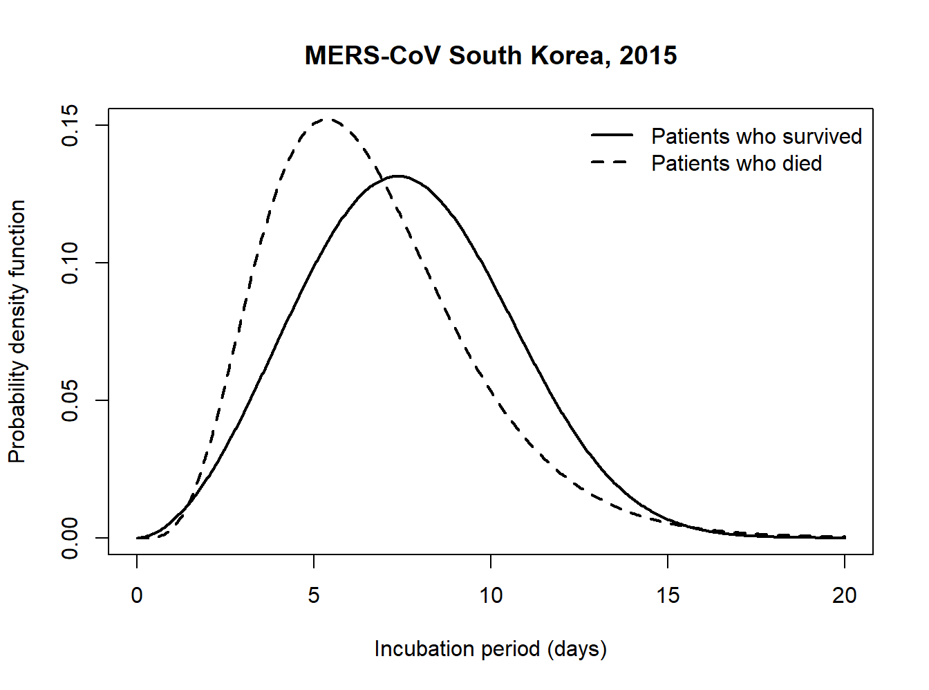
Funding
This work was supported by the ESCAPE project (101095619) and the VERDI project (101045989), funded by the European Union. Views and opinions expressed are however those of the authors only and do not necessarily reflect those of the European Union or the Health and Digital Executive Agency (HADEA). Neither the European Union nor the granting authority can be held responsible for them.
References
Gressani, O., Wallinga, J., Althaus, C. L., Hens, N. and Faes, C. (2022). EpiLPS: A fast and flexible Bayesian tool for estimation of the time-varying reproduction number. PLoS Comput Biol 18(10): e1010618. https://doi.org/10.1371/journal.pcbi.1010618
Gressani, O., Torneri, A., Hens, N. and Faes, C. (2024). Flexible Bayesian estimation of incubation times. American Journal of Epidemiology (Accepted manuscript version). 10.1093/aje/kwae192
Backer, J. A., Klinkenberg, D., and Wallinga, J. (2020). Incubation period of 2019 novel coro- navirus (2019-nCoV) infections among travellers from Wuhan, China, 20–28 January 2020. Eurosurveillance, 25(5):2000062.
Virlogeux, V., Park, M., Wu, J. T., & Cowling, B. J. (2016). Association between Severity of MERS-CoV Infection and Incubation Period. Emerging Infectious Diseases, 22(3), 526-528. https://doi.org/10.3201/eid2203.151437.